One of the most widely used formulas in Excel is VLOOKUP. This formula is used mostly in cases when we need to find something in our range or our table by row. It can also be useful to find duplicates in our files.
We will show how to do this in the example below.
Remove Duplicates Using Vlookup
For our example, we will create a table of NBA teams that participated in the 2020/2021 season playoffs in one column and the 2021/2022 playoffs in another column:
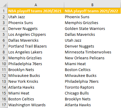
What we want to know now is what teams participated in both playoffs, and which ones did not. The ones who participated in both years will be considered duplicates and will be removed. In column C we will input the following formula:
|
1 |
=VLOOKUP(B2,$A$2:$A$17,1,FALSE) |
This is what the formula looks like in the workbook:
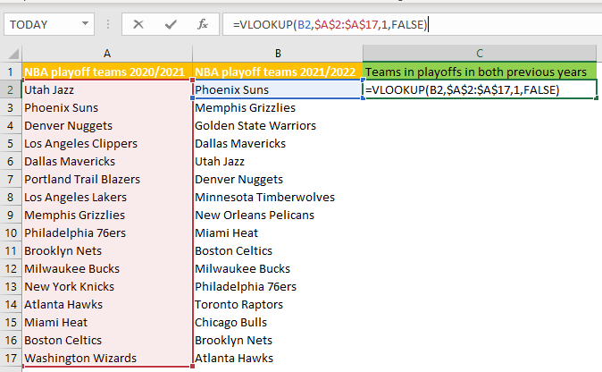
This formula searches for a value in column B (first we search for Phoenix Suns in our case) and it searches this value in column A, and we use lookup FALSE, as we want the exact value to be found.
We have locked data in column A, guaranteeing that, when we change the lookup value, the table array will remain the same.
When we drag and drop the formula to cell C17, this is what we will end up with:
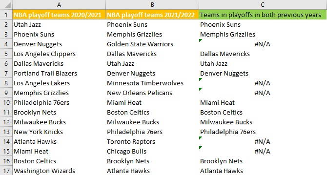
All the teams with a name in column C are the teams that participated in playoffs in the 2020/2021 and 2021/2022 seasons.
Now we only need to filter our data. We will do that by selecting columns A:C and then going to the Data tab >> Sort & Filter >> Filter:

After doing that, we will select a dropdown in column C, and choose all the values except for the “#N/A” values:
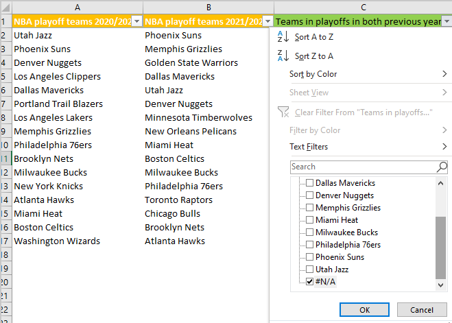
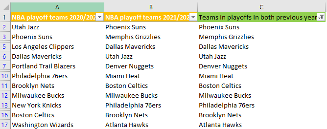
When we do that, we will have only our duplicated values in column C presented:
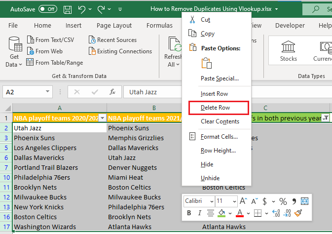
Now we can delete these values by selecting the data, and then right-clicking on them, and choosing the Delete Row option:
After that, we need to clear the filters. We will do that by going to the Data tab >> Sort & Filter >> Clear:

Finally, we will have our data without the duplicate entries, i.e. we will only have unique values presented:

