When you have to work with a spreadsheet that you didn’t create, sometimes you may encounter poorly formatted data or formatting errors.
For example, you open a document, and instead of numbers, you have text values with leading zeros.
Formatting text to numbers won’t work because it will keep zeros at the beginning of the value.
Remove leading zeros and treat values as numbers
Take a look at the following formula.
|
1 |
=VALUE(A1) |
It will convert data into a number and strip zeros in the process.
Take the following data and use it to find out how this function works.
1001001
0100010
0000001
0001000
1000000
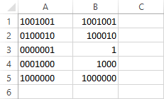
This will return the following result.
CAUTION
When you use somebody else’s worksheet you never know what type of characters there are. Not all of them are printable, so instead of using the =VALUE(A1) function only use =VALUE(TRIM(CLEAN(A1))) to be sure that any unwanted character is not present on your worksheet.
Remove leading zeros and keep values as text
If you want to keep values as text, use the following formula.
|
1 |
=TEXT(VALUE(A1),"#") |
First, it will convert a value to a number in order to delete leading zeros and then it converts it to text with the formatting set in the second argument (#).
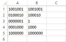
As you can see the result is the same as in the previous example, with the difference that this time the values are aligned to left (default for text).
Delete leading zeros from non-numeric values
The above examples work perfectly as long as we deal with values that can be converted to numbers.
The situation changes when we have numbers mixed with text.
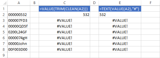
Only the first value is converted correctly, the next cells return the #VALUE error.
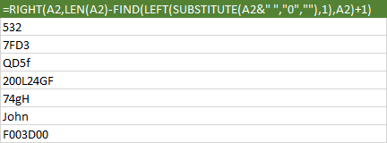
To deal with this problem, you have to use a bit more complicated formula.
Take a look.
|
1 |
=RIGHT(A2,LEN(A2)-FIND(LEFT(SUBSTITUTE(A2&" ","0",""),1),A2)+1) |
Let’s analyze it piece by piece.
|
1 |
=RIGHT(A2,LEN(A2)-FIND(LEFT(SUBSTITUTE(A2&" ","0",""),1),A2)+1) |
This part of the formula will replace all zeros with nothing. This will give us the following result.
|
1 |
=RIGHT(A2,LEN(A2)-FIND(LEFT(SUBSTITUTE(A2&" ","0",""),1),A2)+1) |
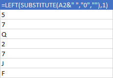
The LEFT function returns the specified number of characters, starting from the beginning of the string.
In this example, it will return the first character of each string.
|
1 |
=RIGHT(A2,LEN(A2)-FIND(LEFT(SUBSTITUTE(A2&" ","0",""),1),A2)+1) |
The LEN function will return the length of the string.

|
1 |
=RIGHT(A2,LEN(A2)-FIND(LEFT(SUBSTITUTE(A2&" ","0",""),1),A2)+1) |
The FIND function returns the first position of the character in the string.
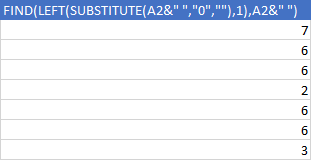
The last function is RIGHT. It returns the specified number of characters from the right side of the string.
|
1 |
=RIGHT(A2,(9-7)+1) |
returns 532.
This is the final result.
