It is nothing unusual to combine a few Excel formulas to get the results we need. Such is the case with the VLOOKUP formula as well.
In the example below, we will show the combination of the VLOOKUP formula and MIN, MAX, and AVERAGE, to extract the desired data in an efficient manner.
Return Min and Max with Vlookup
As you are probably already aware, VLOOKUP has three parameters: 1) Lookup value; 2) Table array and 3) Column index number. There is no limit to choosing a lookup value, i.e. it can be a number, range, or formula as well.
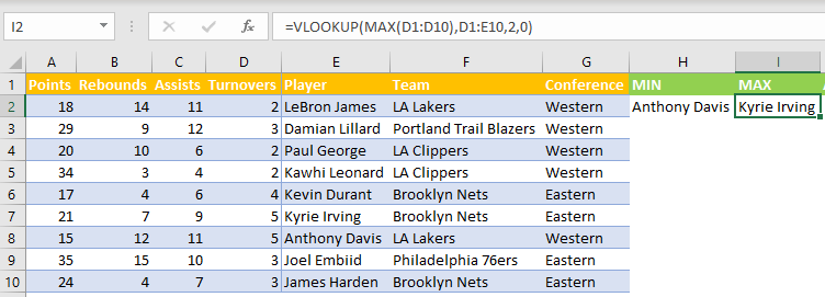
This is where we will input our MIN or MAX formula. For our example, we will use the list of NBA basketball players, their teams, conferences, and statistics from several categories from one night:
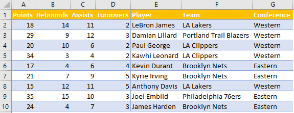
You will notice that the players’ names, their teams, and conference are on the right side of the table. That is the logic that we must follow as it is the way VLOOKUP works.
In columns H, I, and J we will add MIN, MAX, and AVERAGE.
To find the player with the lowest points (MIN) we will insert the following formula in cell H2:
|
1 |
=VLOOKUP(MIN(A1:A10),A1:E10,5,0) |
When we see this formula in our sheet:
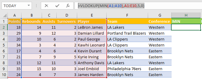
We can notice that our VLOOKUP formula uses the MIN function of column A numbers (range A1:A10, to be exact), and then uses columns A:E as a table array. Since the names of the players have located five spots from points, we use the number 5 as the column index number. For the range lookup, we will choose 0, i.e. to find the exact value.
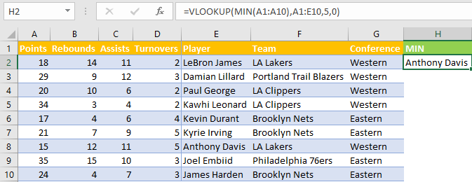
When we click enter, we will get the name of Anthony Davis:
We will use the same principle for getting maximum values for our range. For our example, we will find the player with the most turnovers. We will insert the following formula in cell I2:
|
1 |
=VLOOKUP(MAX(D1:D10),D1:E10,2,0) |
This is what the formula looks like in the sheet:
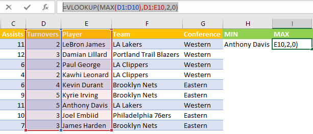
As seen in the table, there are two players with a maximum of five turnovers: Kyrie Irving and Anthony Davis. As Kyrie is the first in our table, his name is the one that will appear as a result:
Return Average with Vlookup
There is a slight difference with using AVERAGE. First, we are going to calculate the average for assists. The result is 8.44. Looking at our table, we will notice that the player with average assists will be either Kyrie Irving or James Harden. When we input the VLOOKUP formula with average:
|
1 |
=VLOOKUP(AVERAGE(C2:C10),C2:E10,3,0) |
Which looks like this in the sheet:
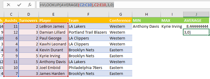 We will end up with the #N/A result. This is because the number 0 in range lookup looks for an exact value, and we clearly do not have a value equal to the average value in our assist column.
To get around this issue, we need to set range lookup to TRUE. This will search for approximate, not exact values. We will change it, and our formula look like this:
|
1 |
=VLOOKUP(AVERAGE(C2:C10),C2:E10,3,TRUE) |
However, we still do not get the expected results, as seen in the following picture:
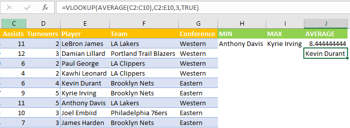
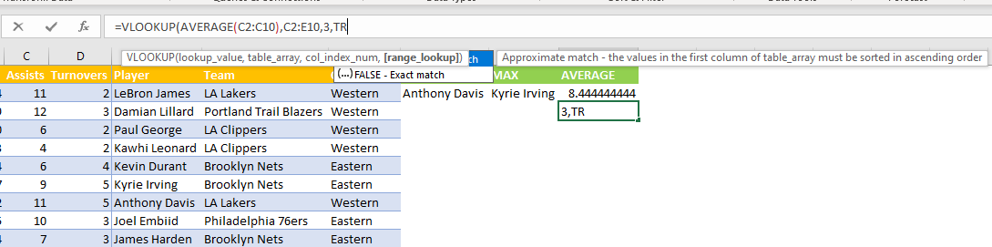
Obviously, Kevin Durant’s assist number (4) is not close to average. The trick here is that we need to have our numbers in ascending order. This is clearly stated when we begin to type TRUE as a range lookup:
So, our solution is to select range A1:G1, then go to Data >> Sort & Filter >> Filter. After that, we will go to our assist column, click on the button, and choose Sort Smallest to Largest:
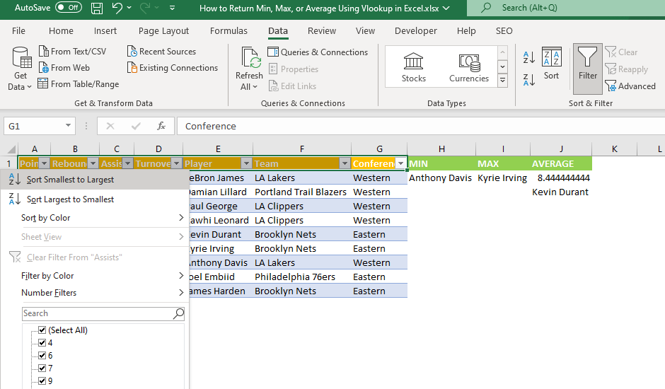
As soon as we do this, we will see that the name of the player that is closest to the average (do remember that it searches for a smaller, not higher value) will be changed and it will now be James Harden:
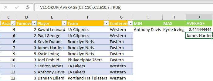
It is seen that, although Kyrie Irving has nine assists, which is closer to our average, our formula will always round to the nearest lower number, and that is the reason we can see James Harden as our result.