We often find ourselves in a situation where we want to have a different view of existing data. As you probably know, Excel has a solution for this as well.
The example below will show how to return multiple values from the table in one cell.
Return Multiple Values in One Cell
For our example, we will use the table with NBA players with several statistics: points, rebounds, assists, and turnovers.
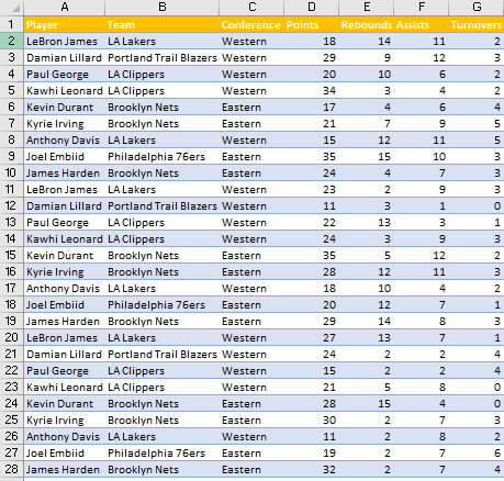
To list out any statistical category for any player, we will use the TEXTJOIN formula.
This formula is only available in Excel 2019 and Excel 365.
What this formula does: it uses and then combines the text from the ranges of your choosing, and then puts up the delimiter you determine between each of the text values that are going to be combined. If you choose the delimiter to be an empty string, it will return multiple values one after the other one.
This formula has several arguments:
- delimiter– We can choose anything to be a delimiter. It separates our text.
- ignore_empty- We choose if we want to ignore cells that are empty or not.
- text1– First range or text value.
- text2– Second range or text value.
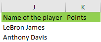
We will prepare the names of the player and define the column points:
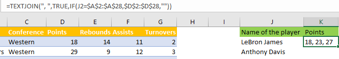
Our formula in cell K2 will be:
|
1 |
=TEXTJOIN(", ",TRUE,IF(J2=$A$2:$A$28,$D$2:$D$28,"")) |
In this formula, we first define our delimiter to be comma and space, i.e. “, ”.
Then we, choose TRUE for ignoring empty cells.
Next, we define our text with the IF formula. The logical test in this formula checks if the value in cell J2 (Lebron James in our example) is the same as in the range of our player’s names- range A2:A28.
This formula goes into every cell in our range and checks if the value is the same or not. If yes, it returns TRUE. If not, it returns FALSE.
The next part of the formula returns all the points that a certain player (located in cell J2 in this case) had in all games. We do that by making sure that the value_if_true part of this formula equals the range where points are found (that is range D2:D28).
So, if the name in cell J2 corresponds to the name in our range, then the points for this player will be presented and will be separated by a comma and space.
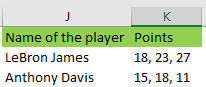
The results are as follows:
All we need to do to apply the same concept for Anthony Davis is to drag the formula to cell K2. Since we have the defined ranges locked, we will get the right numbers:
This formula is different for Excel 2019 and Microsoft 365 users. If you are using Excel 2019, you need to enter the formula, and then hold CTRL + SHIFT, and then press ENTER. The reason for this is that we are dealing with dynamic arrays in this formula.
Microsoft 365 has them incorporated, so all you need to do is input the formula and then press ENTER.