VLOOKUP function is certainly one of the most widely used functions in Excel. Once we extract the data that we want from our original table with VLOOKUP, we can combine it with other options and formulas.
In the example below, we will show how to sort the order in the VLOOKUP function.
Sorting Order in VLOOKUP function
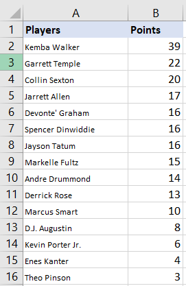
For our example, we will use the list of NBA players and their statistics from one game:
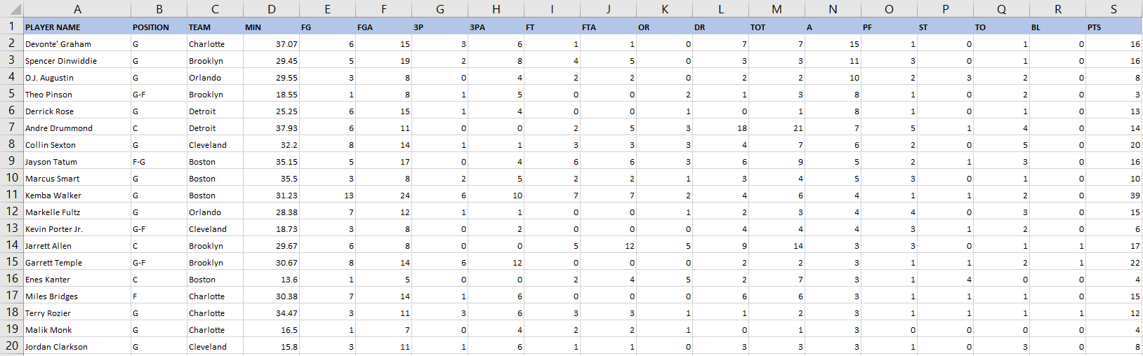
This table is a lot bigger than in the picture, as it has the data for 64 players. In the next sheet, we will copy the first 15 players, and then we will try to find the points that they scored:
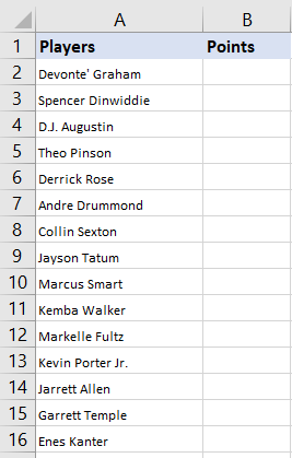
For the next step, we need to find the points for these players from our original table, which is now located in a different, original sheet.
Our formula will be:
|
1 |
=VLOOKUP(A2,'Original data'!A:S,19,0) |
We will drag the formula till the end of our list, or simply double-click on the plus sign that appears once you hover over the bottom-right end of the cell. This is the result we will end up with:
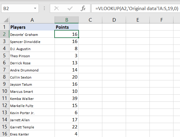
This table imitates the data from our original sheet. As seen in the formula in cell B2, our lookup_value is cell A2, i.e., Devonte’ Graham, while our table_array is the whole scope of the table located in sheet Original data.
The range of the in the table sheet Original data is A:S. For the column number, we choose number 19, because that is where the information regarding points is located in relation to the Players column.
To find out this number, once you choose the table_array, all you have to do is track the number that shows when you choose it, as a helper:

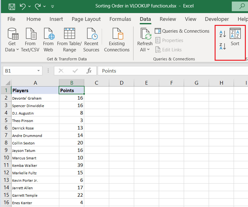
To order the players by points, be it from the smallest number of points to the largest, or vice-versa, all we have to do is click on cell B1 (Points), then go to Data >> Sort & Filter and choose the Sorting option:
We will choose the second option, which is Z to A, or highest to lowest, and this will be our result:
As seen, this sorting has sorted both the players and points.
There is one important thing to remember, though. VLOOKUP function has a fourth, non-mandatory parameter, which is range_lookup. This parameter can be either TRUE or FALSE. If it is set to TRUE (number 1), our formula will look for the approximate value, not the exact one.
FALSE (number 0) searches for the exact value. If we omit this number, we will end up with TRUE as the default value. This will produce some errors and incorrect results in our table:
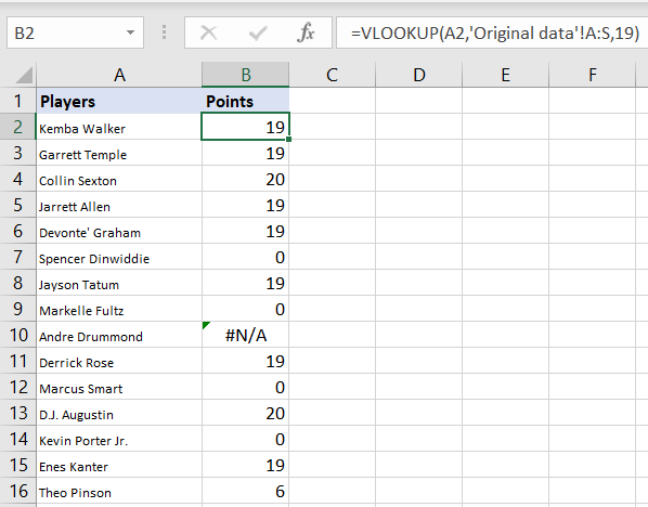
So be careful not to forget to set this value to an exact match, i.e., to 0.