Split Text to Columns With Formulas in Excel

If you want to split the text into columns, you can use Text to Columns Wizard. If you want to have more control over the way you split the text, you can use formulas to do it.

In order to manipulate strings, you can use a few different functions, such as SEARCH, LEN, LEFT, MID, RIGHT, REPT, TRIM, and SUBSTITUTE.

You can create formulas with different combinations of these functions in order to deal with different name combinations, like: first, last and middle name, title, suffix, prefix, etc.

In this lesson, I’m going to create a few formulas for different situations.

There is a great article about it on the official support site.

Text with delimiter

In this part of the tutorial, we are going to use the example with text separated by delimiters.

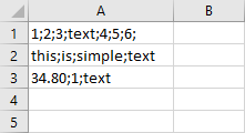
You can split text, using the following formula.

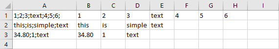
Place it in cell B1 and autofill it to the rest of the cells. The result looks like this.

Analyze the formula

Because there are absolute references to column A1 ($A1) When you autofill the formula, everything stays the same, the only part that changes is COLUMNS($A:A).

First, let’s try the LEN function. It returns the number of characters in a cell.

=LEN($A1) in our case is 17.

Replace this part with the number.

The REPT function inserts a string a specified number of times. In our case, the function inserts 17 spaces. Let’s change the formula.

Let’s analyze this formula.

It will take the string and convert each “;” character to 17 spaces.

"1                 2                 3                 text                 4                 5                 6                 "

The part COLUMNS($A1:A) will return the number of columns. When you autofill the cells it will be:

Formula	Result
COLUMNS($A1:A)	1
COLUMNS($A1:B)	2
COLUMNS($A1:C)	3

The MID function returns the substring from a string given a starting position and length.

If we use this formula.

It will return:

his i

Let’s take a look at what we have for column B1 if we insert this formula.

First element

The first argument in the MID function is a string. In our case, it’s the following string.

"1                 2                 3                 text                 4                 5                 6                 "

The second argument is:

It can be converted (for the first value) to:

1 * 17 - 16 = 1

The third argument is 17. The formula takes 17 characters starting from the first one. This will give us the following substring.

"1                "

Now we use the TRIM function to get rid of any space outside the character leaving us with 1.

Fourth element

Let’s take a look at how it works for the third element.

The fourth column returns 4.

4 * 17 - 16 = 68 - 16 = 52

The formula takes 17 characters starting from position 52, giving us this substring.

"  text           "

Use the TRIM function to get rid of unnecessary spaces.