The SUMPRODUCT function is the combination of addition (SUM…) and multiplication (…PRODUCT). It gets one or more arrays and returns the sum of products of corresponding ranges.
Example:
Take a look at the following example.
Let’s say you want to buy a few things, and you want to know how much money you have to take.
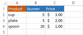
Instead of multiplying the price of each product by the number, and then summing up all the results, you can use SUMPRODUCT to do it all at once.
Use the following formula: =SUMPRODUCT(B2:B4, C2:C4) to calculate the result.
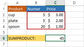
So the result is 45 because 5*3 + 5*2 + 20*1 = 45.
SUMPRODUCT with a single criterion
The function becomes more complicated when we use a condition. But instead of using IF inside SUMPRODUCT, we will use the following notation.
|
1 |
=SUMPRODUCT(--(A2:A5="spoon"),B2:B5,C2:C5) |
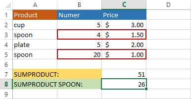
The part (A2:A5=”spoon”) is checking the cells from A2 to A5. If cell equals “spoon” then it treats this value as TRUE, otherwise as FALSE.
We also used double negative (–). It changes TRUE to 1 and FALSE to 0, so we can use multiplication. Alternatively, you can use the following notation.
|
1 |
=SUMPRODUCT(1*(A2:A5="spoon"),B2:B5,C2:C5) |
In the below example, we added another product- “spoon”. Now, we have “spoon” in rows 3 and 5.
SUMPRODUCT with multiple criteria
You can use more than one condition in SUMPRODUCT. Take a look at the next example. We want to count only spoons from the shop in London.
|
1 |
=SUMPRODUCT(--(A2:A5="spoon"),--(B2:B5="London"),C2:C5,D2:D5) |
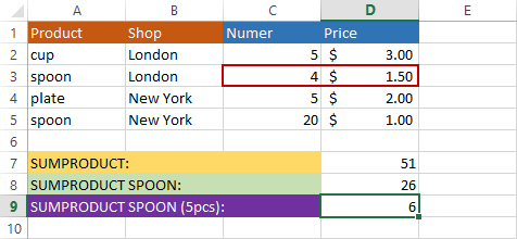
The only product from row 3 is taken into consideration because it meets both criteria.
Multiplication as an alternative to double negative
Instead of the double negative, you can use multiplication, so the formula
|
1 |
=SUMPRODUCT(--(A2:A5="spoon"),B2:B5,C2:C5) |
can be written as
|
1 |
=SUMPRODUCT((A2:A5="spoon") * (B2:B5) * (C2:C5)) |
NOTICE
The second formula uses only one argument.
Advantages and disadvantages of double negative and multiplication
Advantages of multiplication
Multiplication in SUMPRODUCT is more flexible than the double negative. Using multiplication, you can multiply different size ranges. Let’s try the following example.
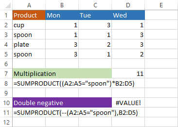
You cannot do the same with the double negative. It will return the #VALUE error.
Advantages of double negative
Take a look at the next example.
The formula
|
1 |
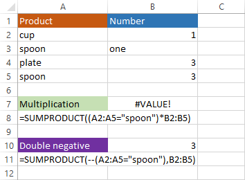
=SUMPRODUCT((A2:A5="spoon")*B2:B5) |
uses cells B3 and B5 to calculate the result. B3 is a text value, and we can’t multiply by text, so the formula returns the #VALUE error.
Double negative ignores this value and returns 3.
Let’s take a look at a bit different example. This time, the multiplication formula also returns the #VALUEerror.
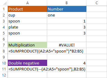
The formula doesn’t even need the value from B2 because it only uses values from cells B3 and B5, but it returns the error anyway.
The double negative returns 4 as expected.
TIP
When you use large sets of data, try to use double negative because it calculates faster.
