Trim and Combine Spaces in Excel

If you import data from legacy systems and external databases into Excel, you most likely will find that the data contains extra spaces.

These extra spaces may be leading, trailing, or between data.

These extra spaces have to be removed because they can cause problems in lookup formulas, printing, charting, and column sizing.

In this tutorial, we will look at the 5 ways of removing and or combining these extra spaces.

Method 1 – Apply the TRIM function

The TRIM function removes all spaces from a text string except for single spaces between words. It deletes all leading, trailing, and in-between spaces except for single-space characters between words.

It was designed to trim only the ASCII space character which has the code value of 32 from text strings.

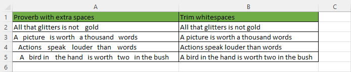
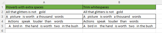
We will use the following example dataset of popular English proverbs to show how the TRIM function can be used to remove extra spaces from data. We have intentionally inserted extra spaces in the beginning, middle, or end of the proverbs.

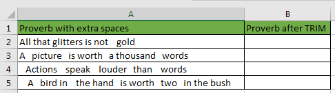
We will do the following steps to remove the extra spaces we have intentionally inserted:

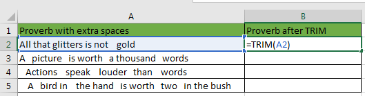
Step 1 – Select Cell B2 and type in the formula =TRIM(A2) as follows:

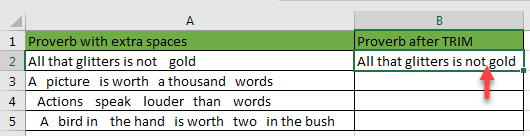
Step 2 – Press the Enter key. You will notice that the extra spaces between the word “not” and “gold” in the first proverb have been removed. Only a single space remains:

Step 3 – Drag down the Fill Handle to copy the formula down the column:

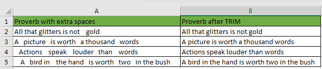
You will notice that all the extra spaces in the proverbs have been removed.

Method 2 – Use the combination of the TRIM function and CLEAN function

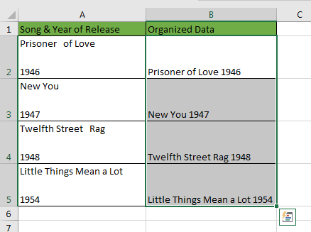
Sometimes the TRIM function alone cannot remove all the extra spaces. This happens when the data has text strings that are broken into different lines like in the example dataset below where the song titles and the years of release are in different lines:

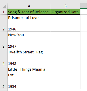
Some of the song titles also have extra spaces.

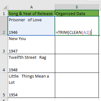
To deal with these issues and make the data more organized we are going to utilize the combination of the TRIM function and the CLEAN function. The CLEAN function removes all nonprintable characters from text.

We will do the followings steps to remove all the unwanted spaces from our dataset:

Step 1 – Select Cell B2 and key in the formula =TRIM(CLEAN(A2)) as below:

Step 2 – Press the Enter key. The line breaks and all the extra spaces have been removed from the first song title and the data is organized:

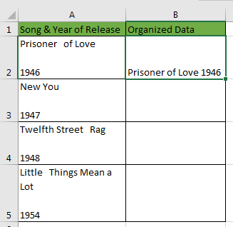
Step 3 – Copy the formula down the column by dragging down the Fill Handle. There are no extra spaces or line breaks in the data and it is now organized:

Method 3 – Employ the combination of the VALUE function and TRIM function

If we apply the TRIM function alone on numeric values it removes the unwanted spaces but returns text strings that we cannot manipulate as numbers for example find their average or sum.

We will have to use the VALUE function to convert the strings back to numbers.

The VALUE function converts a text string that represents a number to a numeric value.

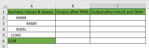
We will use the following dataset of random numbers to show how we can apply the combination of the VALUE function and TRIM function to remove extra spaces from numeric values:

We are going to achieve this by doing the following steps:

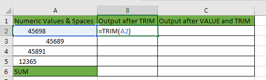
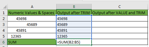
Step 1 – Select Cell B2 and key in the formula =TRIM(A2) as below:

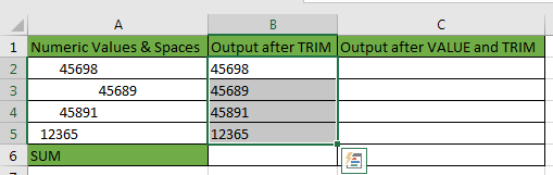
Step 2 – Press the Enter key and drag down the Fill Handle to copy the formula down the column to cell B5. The extra spaces have been stripped from the values:

Step 3 – Select Cell B6 and key in the formula =SUM(B2:B5) as follows:

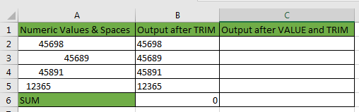
Step 4 – Press the Enter key. You will notice that the SUM function returned a zero because the values in range B2:B5 that were returned by the TRIM function are text values and not numeric:

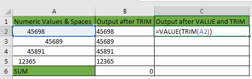
Step 5 – Select Cell C2 and key in the formula =VALUE(TRIM(A2)) as below:

Step 6 – Press the Enter key and drag down the Fill Handle to copy the formula down the column to Cell C5:

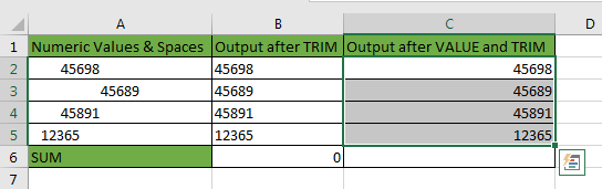
Step 7 – Select Cell B6 and copy the formula to Cell C6 by dragging the Fill Handle across to Cell C6:

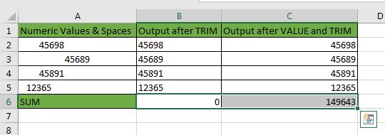
You will notice that the SUM function has returned the correct value because the values in the range C2:C5 are numbers.

Explanation of the Formula

1. TRIM(A2) stripped the numeric value of all extra spaces but converted it to a text string.
2. In VALUE(TRIM(A2)) the VALUE function converted the text string to a numeric value.

Method 4 – Use the combination of the SUBSTITUTE function and TRIM function

The TRIM function removes all spaces from a text string except for single spaces between words. It deletes all leading, trailing, and in-between spaces except for single-space characters between words.

It was designed to trim only the ASCII space character which has a code value of 32.

In the Unicode character set, however, there is an additional space character called the nonbreaking space character. This character is usually used on web pages and has a Unicode value of 160.

This means that the TRIM function which was designed to handle only CHAR(32) space characters and cannot handle CHAR(160) space characters. To handle this kind of space, we will have to employ the SUBSTITUTE function to find CHAR(160) space characters and replace them with CHAR(32) space characters so that the TRIM function can fix them.

We will use the following example dataset to explain how nonbreaking space characters can be removed from data:

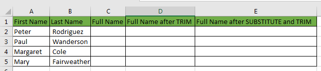
In this dataset, the First Name and Last Name columns have invisible nonbreaking space characters. They however become apparent when we combine the names in Column C.

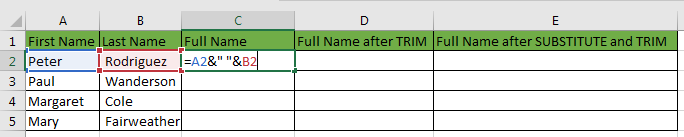
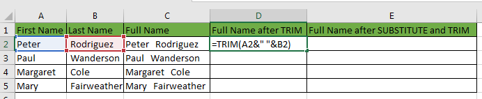
Step 1 – Select Cell C2 and type in the formula =A2&” “&B2 as follows:

Step 2 – Press the Enter key and drag down the Fill Handle to copy the formula down the column:

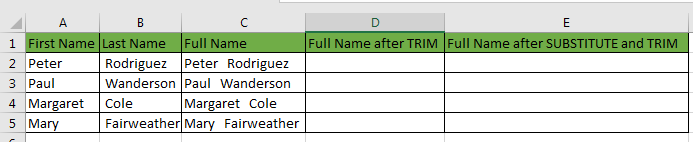
You notice that the full names in Column C have extra spaces. This is because of the nonbreaking character spaces in the data in Column A and Column B.

Let’s see if the TRIM function will remove these extra spaces.

Step 3 – Select Cell D2 and type in the formula =TRIM(A2&” “&B2) as follows:

Step 4 – Press the Enter key and drag down the Fill Handle to copy the formula down the column. The result will appear as follows:

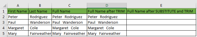
You will notice that the TRIM function has not been able to remove the nonbreaking space characters from the data.

To remove these nonbreaking space characters we have to use the combination of the SUBSTITUTE function and TRIM function.

Step 5 – Select Cell E2 and type in the formula =TRIM(SUBSTITUTE(A2,CHAR(160),CHAR(32)))&” “&TRIM(SUBSTITUTE(B2,CHAR(160),CHAR(32))) as follows:

Step 6 – Press the Enter key and drag down the Fill Handle to copy the formula down the column. The result will appear as follows:

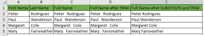
Notice that all the extra spaces in Column E have been removed.

Explanation of the formula

1. In SUBSTITUTE(A2,CHAR(160),CHAR(32)) and SUBSTITUTE(B2,CHAR(160),CHAR(32)) the SUBSTITUTE function replaces the nonbreaking space characters in Cell A2 and Cell B2 with ASCII space characters. The nonbreaking space characters are represented by code value 160 and the ASCII space characters are represented by code value 32.
2. The extra space characters are then removed by the TRIM function.

Method 5 – Free Excel Add-in for SEO

If you don’t want to use functions and formulas, you can use a free add-in that can trim and combine spaces.

After you install the plugin and select the text you want to manipulate, you can navigate to SEO >> Text >> Trim and Combine >> Trim Spaces.

All whitespace from the beginning and the end of the sentences are removed.

But there are still multiple spaces between words. For this reason, we are going to use the next button, called Combine Spaces.

After you click it, multiple adjacent spaces are combined into one.