VLOOKUP by Column Name in Excel

Most of the things that people use in Excel can be combined to achieve proper and adequate results. Using the VLOOKUP function is not any different from this. We can use it in a combination with another formula to achieve the VLOOKUP by Column name.

We will do this in the example below.

VLOOKUP by Column Name in Excel

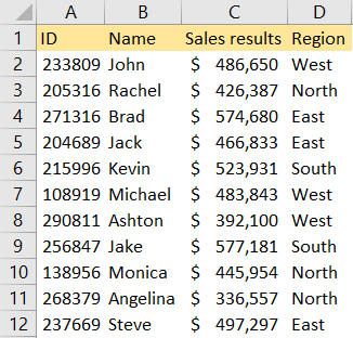
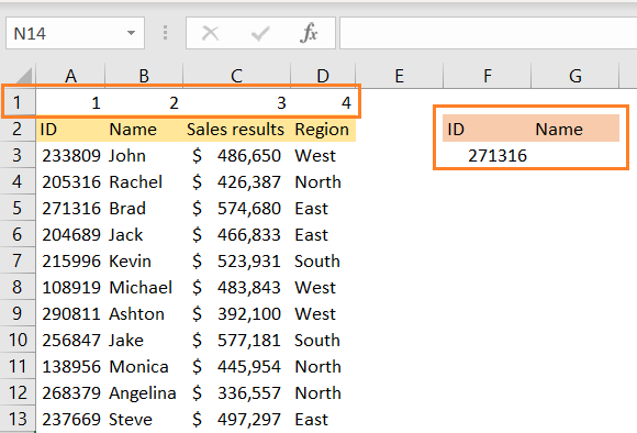
For our example, we will use the list of salespersons, their company IDs, sales results, and the region that they are located in:

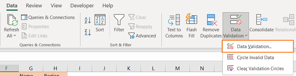
Now, there is a cool option for choosing the IDs and then going automatically getting the results in a table. For this, we will use Data Validation. We will go to the desired cell, in our case, cell F2, and then will go to Data >> Data Tools >> Data Validation:

On the window that appears, we will choose the List in Allow tab, and our source will be the list of IDs:

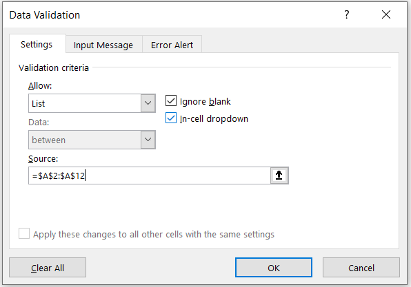
This way, we will have our IDs in the dropdown in cell F2.

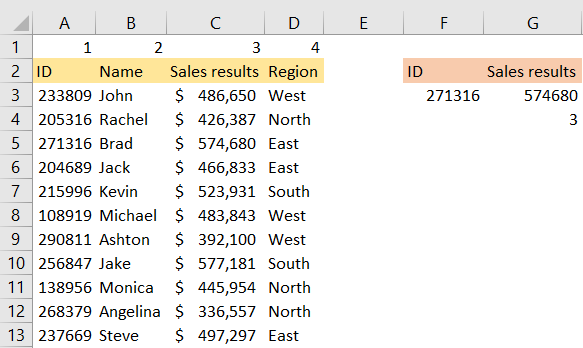
We will add the Name column next to our ID. After that, we will insert another row before the first row (helper row), and will add numbers to the fields:

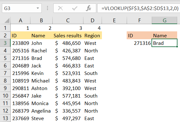
It is pretty easy to use VLOOKUP and to find out the name of the person on our table with ID 27316. To achieve this, our formula will be:

In the formula above, we lock the F3 cell (our lookup value), and we also lock our table array to be range A2:D13. Our column index number is number 2, as we want to find out the name of the salesperson. This will be our result:

What we want to achieve at this point is to change the value in cell G3 by changing the value in cell G2. For example, we know that Brad works in the East region, but if we would simply put the Region in cell G2, nothing would happen:

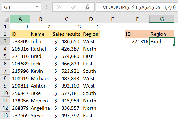
This is why we have our helper’s row, and it will come in handy. We need to replace the column row index with the MATCH formula.

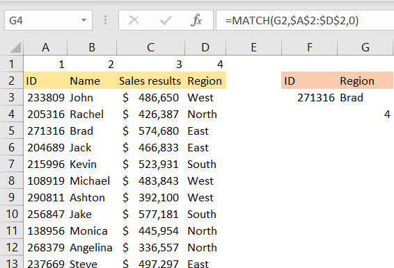
We will insert this formula first beneath our existing VLOOKUP formula. This is the formula that we will put into the cell G4:

Our MATCH function searches for the value located in cell G2, in the array A2:D2. We can expect the result to be number 4, as that is where our value is located in the range (at place number 4):

All we need to do now is to replace the column index number in the VLOOKUP formula with our MATCH formula. So, we will copy the MATCH formula in the VLOOKUP formula, and end up with:

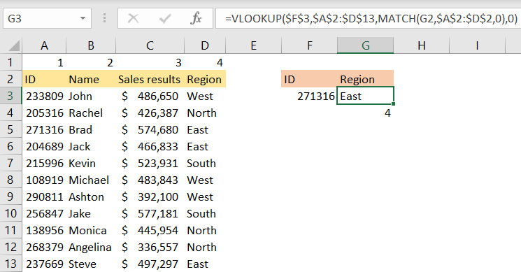
Now we can easily change the value in cell G2 to some of the values in our column names and be sure that we will get exact results. If we change the value for Sales results, we will get number 574,680, which is the results Brad achieved: