The AutoSum feature is used to sum the values of columns or rows with a single click. When you use it, Excel tries to guess which cells you are trying to sum up. I’ll show you a few methods to use this tool and explain when you have to be careful if you want to avoid problems.
There are three places where you can access the AutoSum feature.
1. HOME >> Editing >> Autosum,
2. FORMULAS >> Function Library >> AutoSum,

3. Using the Alt + = keyboard shortcut.
Example 1:
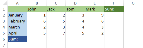
In the following example, there is a table with four names in the header. The table contains the number of points scored by each person each month.
Let’s sum up the points for January. Click cell F2 and press the AutoSum button.
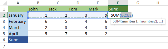
Excel will highlight the cells that will be summed up. Press Enter to confirm.
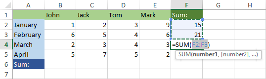
Do the same for February. To do this, click cell F3 and then use AutoSum.
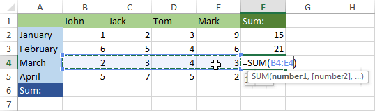
Try the same for March (F4). This time when you click AutoSum, this time Excel will choose the cells above the currently selected ones, instead of those that are located to the left.
Since you have more than one value above the selected cell, Excel decides to sum the column, not the row, as it did before.
To correct Excel, select cells (B4:E4) and press Enter.
Summing everything at once
After you sum up points for April, you can count the totals for each person. To speed up your work, we will use the AutoSum feature to sum up all these cells with one click.
First, you need to delete all the unnecessary cells to restore the example to its original state. After you do this, select cells from B2 to F6 and click the AutoSum button.
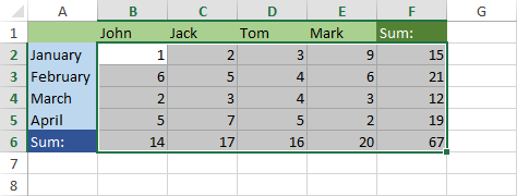
As you can see Excel summed up rows, as well as columns.