When dealing with Excel tables, we can often forget how naming conventions and their grouping can be useful in our work.
In the example below, we will show how to use the table names and to reference them easier in different sheets in our workbook. We will then show how to dynamically reference table names, i.e. keep the reference to the table in different sheets while changing the table name itself.
Using Indirect Formula to Reference Tables
For our example, we will create three tables that will show sales results from three top salespeople of every branch.
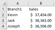
First, we will create a simple list, as shown below:
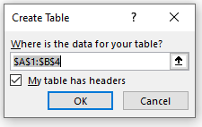
Then, we will select our data, and go to Insert >> Table. A pop-up window will appear, and it will ask us again to confirm our range:
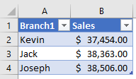
When we click OK, our table will be created:
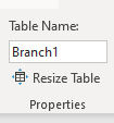
To define the table name, we need to click anywhere on the table, and then go to the Table Design tab. Once there, we will go to Properties and change the name of our table to be Branch1:
We will do this for other branches as well and we will have three branches as a result:

Next thing, we will create another sheet which we will simply call the „Indirect formula“ since this is the formula we are about to use.
We will click on cell B1, go to and then go to Data tab >> Data Tools >> Data Validation:
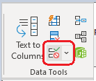
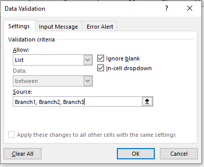
When we click on it, we will be directed to the Data Validation pop-up window. On this window, we will choose List beneath the Allow option, and we will input the names of our tables (Branch1, Branch2, and Branch3) in the Source part:
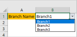
When we click OK, you will notice that we created a dropdown in the cell B1:
In the fourth row, in cell B4 we will input the following formula:
|
1 |
=SUM(INDIRECT(B1)) |
This formula will SUM the numbers in the table that we will choose in cell B1. For our exercise, we will choose Branch2:
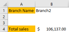
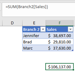
You will notice that we are presented with the number of $106.137.00. This is the same number that we would get if we summed all the sales for Branch Number 2 in the first sheet:
So, with the Indirect formula, we can dynamically reference our tables in different sheets, and use the various formulas (MAX, MIN, SUM, etc.) to get the results that we want from our original table.
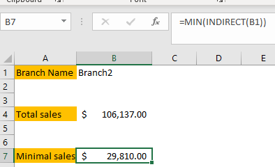
For example, we will use input the MIN formula in a combination with INDIRECT in cell B7:
|
1 |
=MIN(INDIRECT(B1)) |
We will get the following results:
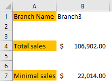
The beauty of this formula is that we only need to change the cell B1 to derive the same results but in different branches:
Dynamically Reference the Tables
The problem that we now have is that- any user can change the names of our tables. In that case, our list in sheet “Indirect formula” will be worthless.
Luckily, there is a solution for this problem as well, and it can be resolved by adding formula through VBA.
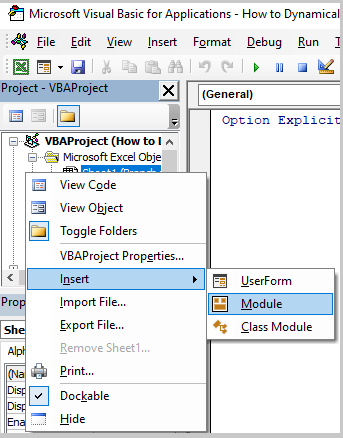
To do this, we will open our Module in VBA by clicking ALT + F11 and then inserting Module by right-clicking on the left window:
Once we have our Module, we will input the following formula in it:
|
1 2 3 4 5 6 7 |
Function TableName(cell As Range) As String Dim Name As String Name = vbNullString On Error Resume Next Name = cell.ListObject.Name TableName = Name End Function |
This function looks like this in our module:
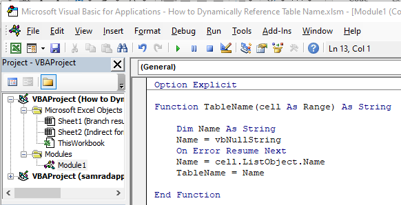
What it does is it first creates a function called “TableName” with one parameter called a cell, which will be defined as a range. The whole function will be formatted as a string, as we need to return the name of the table:
|
1 |
Function TableName(cell As Range) As String |
For the next thing, we declare the „Name“ variable as a string and we define it to be equal to a null string. This is a constant that denotes the null string.
We define that if we have the error we should ignore it:
|
1 2 3 |
Dim Name As String Name = vbNullString On Error Resume Next |
For the last part, we define the „Name“ variable to be equal to the name of the object where our cell is located (we need to point out to any cell in our table to retrieve the name of our table in the worksheet), and then we finally declare our TableName to be equal to the cell we retrieved:
|
1 2 |
Name = cell.ListObject.Name TableName = Name |
We will change the name of our first table to Branch148 in table properties. Then, we will call for our formula and point to any cell in the first table (in this case cell B2):
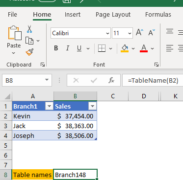
We will do the same for table 2 (renamed to Branch 422) and table 3 (renamed to Branch 512). We will get the following results once we apply our formula:
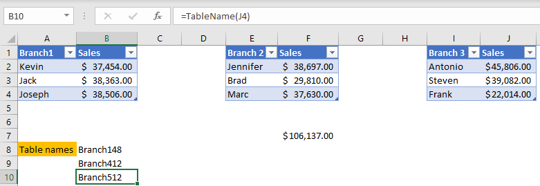
For the last step, we need to go to the sheet “Indirect formula” and change the scope of the Data Validation as follows:
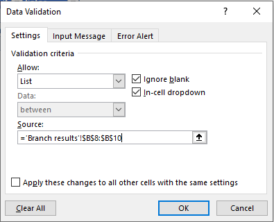
Now, if we do happen to change the name of our tables in table properties, we have the formula that will generate this change, and we have the data validation that will always get the data from the cells where our formula is applied.
In this way, we dynamically referenced table names.
