So far, you are probably aware of the good things and improvements in your daily activities that VBA can bring.
When talking about multiplying cells in Excel, it is no different. Multiplication itself is not easy to be shown on one example, as there are limitless options: multiply two numbers, multiply many numbers with many numbers, multiply one number with multiple numbers, and so on.
We will cover one of these options below.
Multiply range of cells using Absolute Referencing
For our exercise, let us presume that we have the following numbers and multiplier in our table:

Our goal is to write the code that will automatically multiply numbers in column A with a multiplier in cell B2, and finally, show the results in column C, in the correct order. This means that the result of A2*B2 should be in cell C2, the result of A3*C2 should be in cell C3, and so on.
For writing the code, we first need to access the VBA. To access the VBA, you can go to Developer tab >> Visual Basic:
You can also simply click ALT + F11.
Once we do, we will get the Visual Basic window, on which we will right-click on the left window, and choose Insert >> Module:
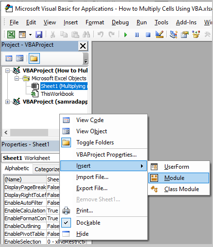
We will be presented with the blank sheet on the right side, and on it, we will input the following code:
|
1 2 3 4 5 6 7 8 9 10 11 12 13 14 15 |
Sub Multiply_Range_with_Number() 'Declaring variables Dim numbers As Range, multiplier As Range Dim a As Range Dim c As Integer 'Setting variables Set numbers = Range("A2:A" & Range("A65000").End(xlUp).Row) Set multiplier = Range("b2") c = 2 'For each loop For Each a In numbers Cells(c, 3) = a * multiplier c = c + 1 Next a End Sub |
This is what this code looks like in VBA:
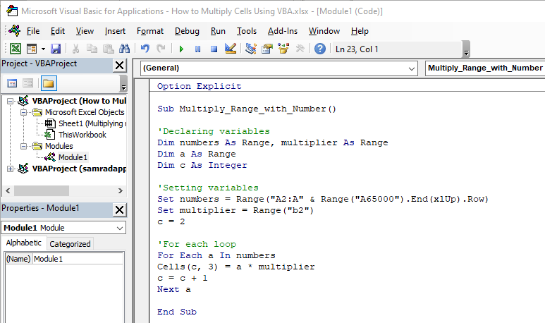
This code has three parts, and these parts are found under the comments (comments in VBA are written by using “ ’ ” before the text that we want to write.
The first part of the code declares the variables that will be used. The declaration is a term that is used to show that we need a certain variable. Once we declare them, we need to assign them to a certain value.
The numbers value refers to the range in column A. Our multiplier is in cell B2 (number 2). We add another variable- variable c, that will be initially set to be number 2 (presenting row number 2 in later code).
The last part of the code takes our variables and puts them in the For Each Loop:
|
1 2 3 4 |
For Each a In numbers Cells(c, 3) = a * multiplier c = c + 1 Next a |
It states that each cell located in column A (populated cells) takes that value and places it into row 2 of column 3. Then it takes the value from column A and multiplies it with our multiplier.
To secure that we move to another row in column C, we add this part:
|
1 |
c = c + 1 |
This means we will now be positioned in cell C3 when we execute the loop again, and cell C4 the next time, and so on.
We also move in column A every time with the “Next a” part of the code.
We can execute the code by clicking F5 or by clicking the green button in the module:

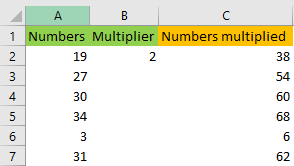
Once we click on it, we will see the results in our table:
Multiply the range of cells using Relative Referencing
The above approach to doing things is absolutely fine. But what we want now is not to have the range hardcoded, i.e. we want our users to be able to choose the range where the original numbers are located, where the multiplier is, and where they want to have the results shown.
To do this, we need to tweak our code a little bit. Our code will look like this:
|
1 2 3 4 5 6 7 8 9 10 11 12 13 14 15 16 17 18 19 20 21 22 23 24 25 26 27 28 |
Sub Multiply_Range_with_Number_2() 'Declaring variables Dim numbers As Range, multiplier As Range Dim a As Range Dim c As Integer Dim d As Long 'Setting variables Set numbers = Application.InputBox( _ Title:="Numbers that need To be multiplied", _ Prompt:="Select the numbers that you want To multiply", _ Type:=8) Set multiplier = Application.InputBox( _ Title:="Multiplier", _ Prompt:="Select where your multiplier Is located", _ Type:=8) c = 2 d = Application.InputBox( _ Title:="Column in which results are stored", _ Prompt:="Select the column For storing the results", _ Type:=1) 'For each loop For Each a In numbers Cells(c, d) = a * multiplier c = c + 1 Next a 'Defining cell name Cells(1, d) = "Results" End Sub |
This is what our code looks like in the module itself:
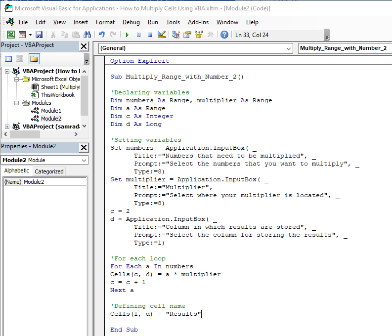
As you can see, the code is pretty much like the one presented in the first example. The difference here is that we do have one more variable- variable d as long.
The difference is also that we are setting every variable (except variable c) with the Application.InputBox method.
With it, we are asking users to choose the original range, the multiplier, and the column in which the results will be stored.
The type for the first two Application.InputBox formula is 8, which means this refers to the range, and for the third, it is 1, which means we refer to the number.
We have two more additions to our formula- we added the variable d in our For Each Loop as well, and we define the first cell of the column where the results are stored to be “Results”.
Once we execute the code, we will get the three messages (for three variables) as follows:
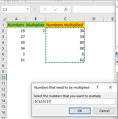
First, the user is asked to select the numbers for multiplication. We have chosen numbers in the C column, and then we click OK.
Next, we are asked to choose our multiplier:
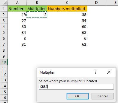
Remember, we need to choose the actual cell (range) as this variable is defined as a range. If we simply typed in the number 2, we would get an error message.
Finally, we click OK, and are asked to insert a column in which we want to store the results:
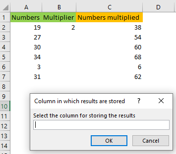
In this step, we need to insert an actual number, rather than a cell, as we defined this variable as a number.
Of course, you could have typed in these instructions for the user as well.
We will insert number 4 (column D), click OK, and finally have our results:
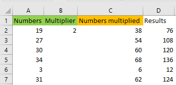
You will notice that cell D1 is also populated with the text “Results”, as defined. Pretty neat, right?