We have explained a lot of work that can be done in Excel with Pivot Tables. But, as every part of this program has continuous development, there will always be a need for more learning and/or for updating existing knowledge.
One of the things that can certainly help is to explain how to add a column to a Pivot Table that will be a percentage of an existing column. We will show how to do this in the example below.
Add Percentage Column in Pivot Table
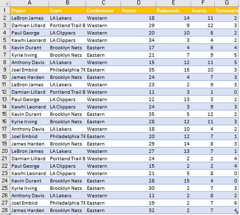
For our example, we will use the table with NBA players and their statistics for three nights, for several categories: points, rebounds, assists, and turnovers:
We will create a Pivot Table, we will simply select our whole table (to do this, we can either click and drag on it or position ourselves to the first cell (cell A1) and then click the combination of CTRL+SHIFT+LEFT and CTRL+SHIFT+DOWN.
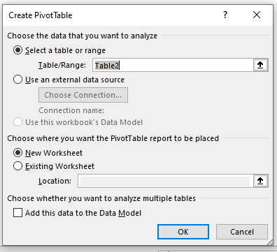
When we do this, we will go to Insert >> Tables >> Pivot Table. We will simply click OK on a pop-up that appears:
Our Pivot Table is created in another sheet, and we will call this sheet simply Pivot Table.
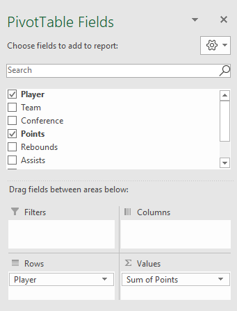
We will now put Player in Rows field and Points in Values field (we will use SUM function):
We know that we have statistics for three nights, and we also realize that, if we want to find out the percentage of points, we need to divide the sum of points with the number three.
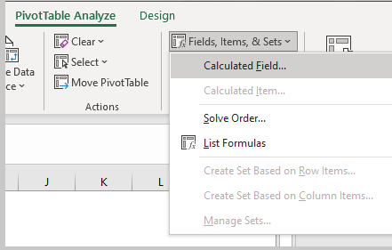
To add this column, we will click anywhere on our Pivot Table and go to the tab PivotTable Analyze >> Calculations >> Fields, Items, & Sets >> Calculated Field:
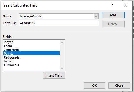
On a pop-up window that appears, we will change the name of our column to be “AveragePoints”, and then insert the points field and divide it by 3:
When we click OK, we will have another column inserted:
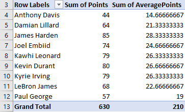
You will notice that Excel makes a little mistake here. As this column is automatically inserted in the Values field, it gets the custom name starting with “Sum of”. However, we know that this number refers to the average of points. If you want to change this, you have to do this manually.
The second problem that we do have now is that we cannot format these numbers to have the percentage sign, as we will have numbers formatted as 1900%, instead of 19% for the last number.
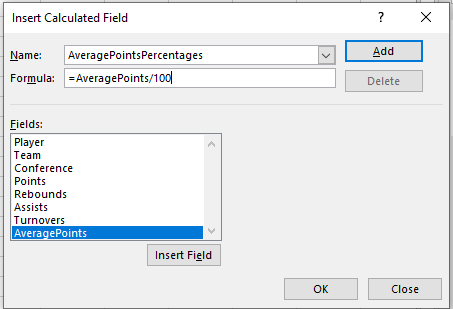
To do this we will create another field which will be the created field divided by 100.
We will click OK and have the following results:
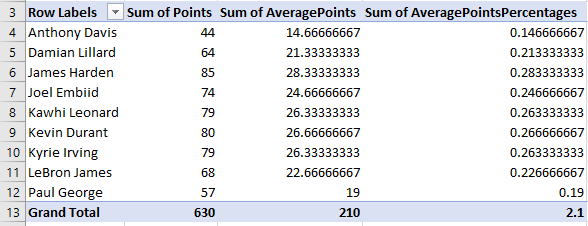
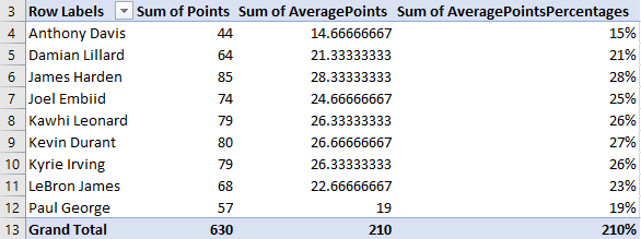
We will select this column, go to the Home tab and click on the percentage sign:
Finally, we have a nice percentage column in our Pivot Table: