Use COUNTIF with Conditional Formatting in Excel

We have already shown how useful and helpful conditional formatting can be. To make things more interesting, conditional formatting can be used in a combination with various formulas, to highlight desired cells.

We will show how to use conditional formatting with COUNTIF and COUNTIFS in the examples below.

Conditional Formatting with Countif

COUNTIF is a useful function that counts the number of times cells that have some certain parameter appear in a range.

It has two parameters:

Range – The range in which we are searching for the desired word, number, or phrase.

Criteria – The criteria itself that a cell in a range has to contain to be counted.

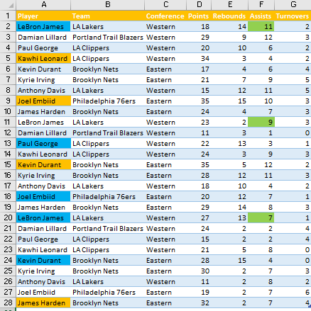
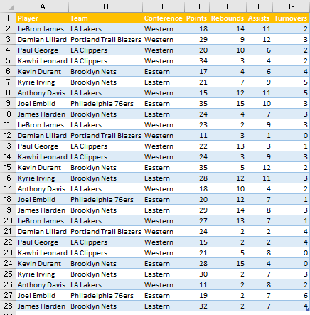
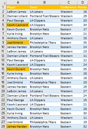
To show how to combine this formula with conditional formatting, we will use the list of NBA players and their statistics from a couple of nights.

For the first example, let’s suppose that we want to highlight only the assists from LeBron James. We can do this by using the COUNTIF function.

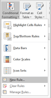
We will select column F (as the assists are located in this column) and go to Home >> Styles >> Conditional Formatting >> New Rule:

On a pop-up window that appears, we will select the last option- Use a formula to determine which cells to format:

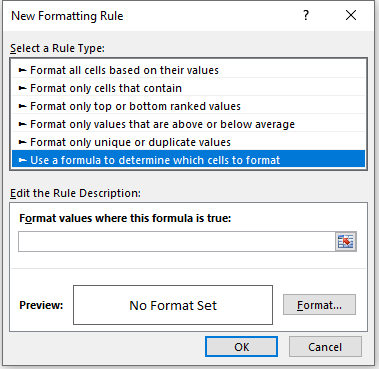
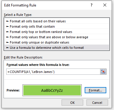
We will input all our formulas in this little box beneath the text: “Format values where this formula is true:”

Our first formula will be:

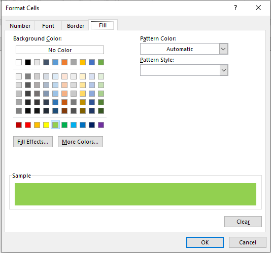
We have to select the range where our desired criteria are found, which is column A. For that reason, we choose cell A1, to order the formatting correctly. Then we will click format and choose the Fill tab and green color:

Our formatting rule preview will look like this:

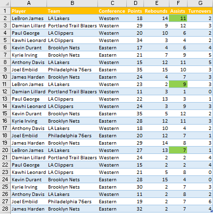
When we click OK, we will see changes in our table:

We can also have several criteria to highlight the desired cells. For example, let’s say that we want to highlight all the players that had more than 30 points.

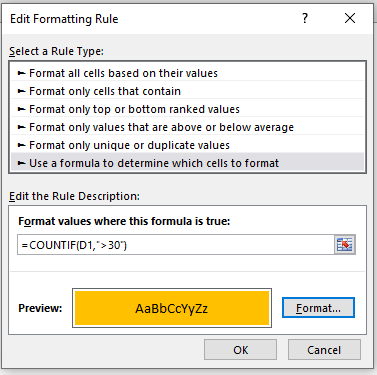
To do this, we will select column A and follow the same steps in the first example. Only our formula will change and now it will be:

When we input the formula in the Edit Formatting Rule window and declare these values to be filled with orange color, our window will look like this:

Our first column will now have all the players that put up more than 30 points highlighted in orange:

Conditional Formatting with Countifs

COUNTIFS works on the same principle as COUNTIF, with the difference it observes multiple criteria instead of just one.

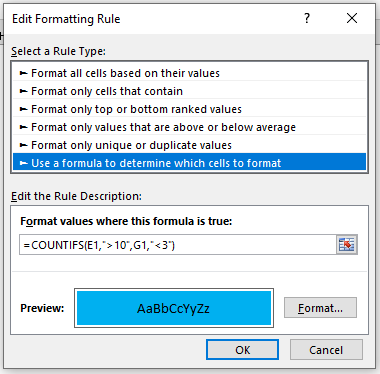
So we will use COUNTIFS to find all the players that had more than 10 rebounds and less than 3 turnovers.

Our formula will be as follows:

And our pop-up window will look like this:

All other steps are the same as in previous examples. Our table finally looks like this: