Excel has many formatting options for numbers, fonts, and everything else we might need and use. Using them is not always self-exploratory, but that does not mean there is no way to achieve something.
In the example below, we will show how you can format the date with a line break in Excel.
Date Format With Line Break in Excel
When we want to insert a line break in our cells, we use a combination of ALT + ENTER. This will be the result:
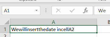
We can read “We will insert the date in cell A2” but it looks funny and unreadable. To make it better, we will select the cell, and then choose the Wrap Text option in Alignment:
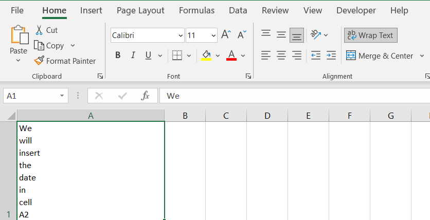
If needed, we will expand cell A1, and the text will appear.
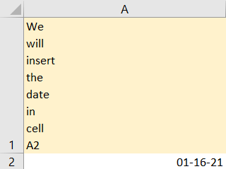
The same approach we use for this will be used for formatting dates. In cell A2, we will insert the date January 16th, 2021:
To format this date with line break, we need to select it, then either right-click on it and choose Format Cells, or find the number formatting option in the Home tab. We will choose the first option:
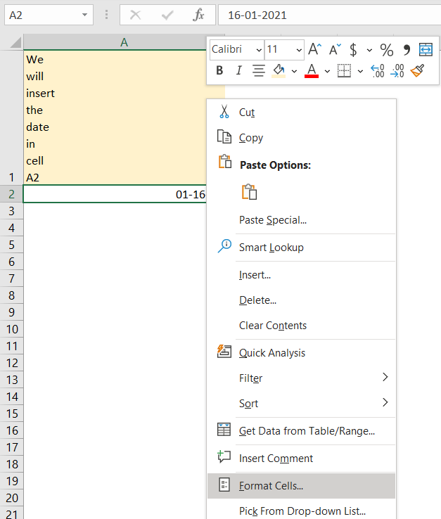
In the dialog box that appears, we will choose Custom in the Number tab, then insert “dd” under Type, followed by CTRL + j (this will allow us to write in the next line under Type), then we will type “mm”, followed by another CTRL + j, and finally, we will type “yyyy”. This is what our sample will look like:
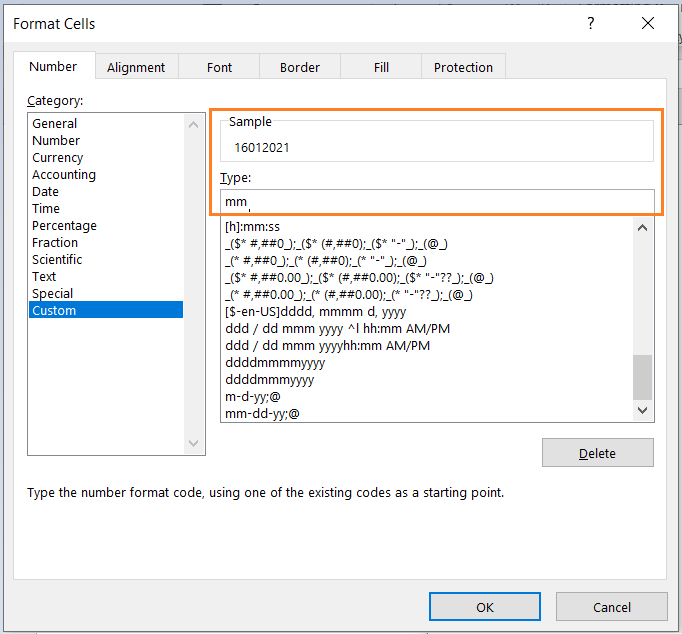
When we click OK, we will have the numbers written in cell A2, but in this funny format:
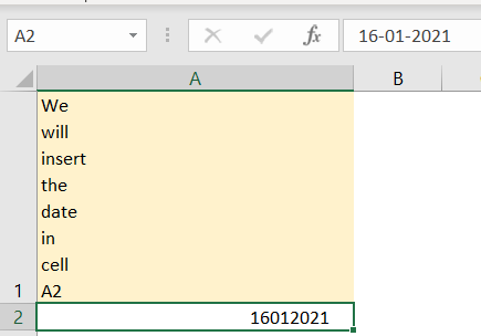
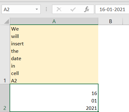
In the formula bar, we can notice that the date still remains the same, which means we need to use the same approach- select the cell, choose Wrap Text, and then expand cell A2. This is our final result:
