Some characters that we may want to include in a cell in Excel are special characters in that they are used by the application itself. The characters have a special functionality within Excel.
Examples of the special characters are the full colon (:) that is used for formatting time values and double quotes (“) that are used to mark the beginning of the end of text-only arguments of functions.
Different Escape Techniques We Can Use in Excel
To include the special characters in a formula or some other input value in Excel, we need an escape technique that tells Excel that we want to include these characters in the value or formula we are inputting and that we do not want them to be interpreted in Excel’s default manner.
When we escape a special character, we are telling Excel to treat the character as literal text.
In this tutorial we are going to look at the following 6 methods that we can use to escape special characters in Excel.
Method 1: Use Additional Double Quotes inside a Formula
In the Excel default settings, double quotes are used to mark the start and end of a text string.
If we want to include double quotes inside a formula value, we can use additional double quotes in the formula.
We will use the following example to show how this is done:
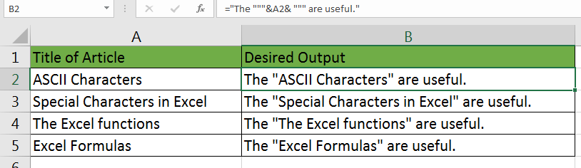
In the example, the formula in cell B2 is:
|
1 |
="The """&A2& """ are useful." |
The outer quotes (1 and 4) tell Excel that this is text, and the second quote tells Excel to escape the next character and thus the third quote is displayed.
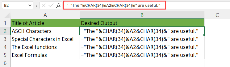
Method 2: Use the CHAR Function With the Code Value 34
Since double quotes (“”) can also be used for an empty text string, the use of double quotes in formulas can get confusing so another way to achieve the same results is to use the CHAR function with the code value 34.
The CHAR function returns the character specified by a valid code number.
In the following example, the formula in cell B2 is =”The “&CHAR(34)&A2&CHAR(34)&” are useful.”
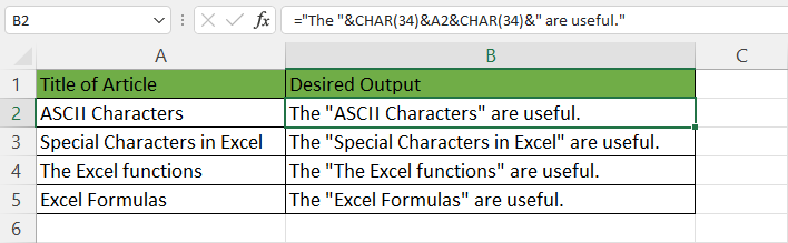
In this example, CHAR(34) returns the double-quote character which is included in the output as literal text.
Method 3: Use the backslash (\) in a Custom Number Format
We can use the backslash (\) character in custom number format in a cell to escape special characters like a colon (:).
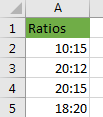
The following example shows a list of ratios:
To achieve this display, we have to escape the colon character by creating a custom number format as follows:
- Press Ctrl + 1 to open the Format Cells dialog box.
- In the Type box type in #\:## as follows:
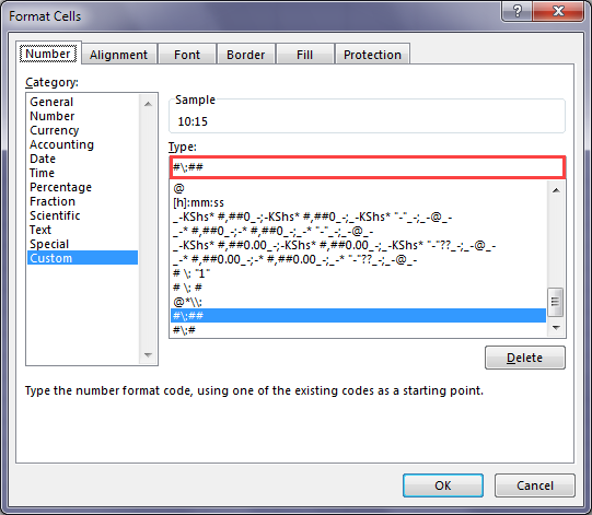
With this custom number format, 1015 will be displayed as 10:15, 2012 as 20:12, and so on.
If we want to display single-digit ratios for example 4:2, 1:1, we have to enter the custom number format as 0\:0 in the Type box.
Using the backslash character is equivalent to wrapping the next character in double quotations.
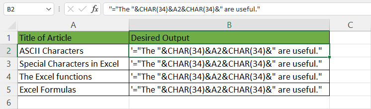
Method 4: Use an Apostrophe (‘) at Beginning of the Formula
The equal sign (=) is used to start the formula in Excel, and it can also be used to compare values.
Sometimes we may want our formulas with the equal sign to be displayed as text and not to be evaluated by Excel.
We achieve this by preceding the formula with an apostrophe (‘) character. Like in the following example:

The formula in cell B2 is preceded with an apostrophe character as:
|
1 |
'="The "&CHAR(34)&A2&CHAR(34)&" are useful." |
The apostrophe character tells Excel to treat the formula as text. The character is not displayed in the cell, but it can be seen in the formula bar:
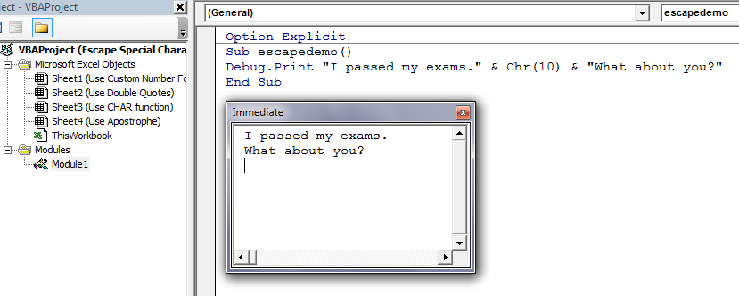
Method 5: Use the Chr function in Excel VBA
In Excel VBA we use the Chr function to escape characters. This inbuilt function returns the ASCII equivalent value of any valid code number from 0 to 127 that is passed to it.
In the following example the Chr function returns a linefeed character:
Method 6: Double the Apostrophe (‘) Character
The apostrophe causes Excel to interpret the value entered in a cell after it as text instead of a number or formula.
If we want to include the apostrophe character in the formula output, we have to double it as in the following example:
The formula in cell B2 is preceded with double apostrophes:
|
1 |
''="The "&CHAR(34)&A2&CHAR(34)&" are useful." |
The apostrophe is now displayed in the data because the first apostrophe tells Excel to output the second apostrophe as text and not as a special character.
Conclusion
In this tutorial, we have looked at 6 different methods that we can use to escape special characters in Excel.
When we “escape” special characters in Excel, they are interpreted differently from their default behaviour by Excel and not with their special meaning. We override the default behaviour of Excel and display values the way we want.
We have looked at the use of additional double quotes and the CHAR function. To override the default behaviour of double quotes (“”) in a formula, we use additional double-quotes. We use double quotes to escape double quotes. Alternatively, we can achieve the same results by using the CHAR function with an argument of code value 34.
We also looked at preceding a formula with an apostrophe. To escape the equal sign (=) character we precede the example with an apostrophe (‘) character. This tells Excel to treat the formula as text.
We saw that the apostrophe (‘) character tells Excel to treat the value that follows it as text and not a number or formula. Therefore, if we want to include it in the formula output, we have to double it (”).
The use of the backslash (\) character in a custom number format can also be used to escape special characters in Excel.
In Excel VBA we use the Chr function to escape characters.
Each of the methods has its strengths and weaknesses and generally, we will have to use a combination of the methods to achieve the results we seek.