Excel is one of the most widely used tools for presenting data. Having this in mind, it often comes down to the way of presenting it, not just the data itself.
Users often find themselves having problems with formatting. In the example below, we will show in which way can you format your row numbers to present the data in the way you want.
Existing Formatting Options
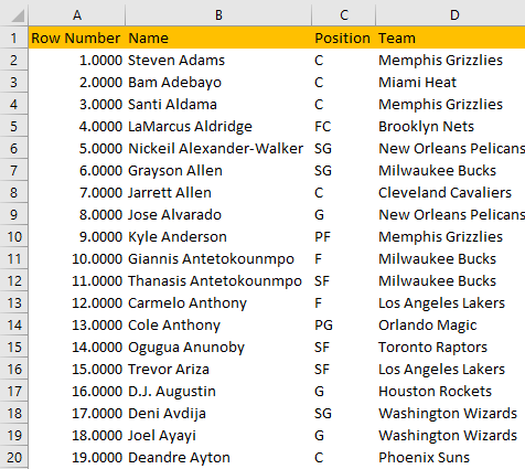
For our example, we will use the list of NBA players, their positions, and their respective teams:
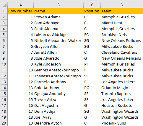
We have added row numbers to distinguish these players. Since we did not define these numbers, they will be formatted as General type. This is the default format of all numbers that Excel applies. Usually, numbers that are formatted in this way are displayed in the same way in which they are typed.
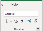
If we want to change this format, we have several options. Mostly used is that we select our range, then go to the Home tab, and then on the little icon right to the word Number:
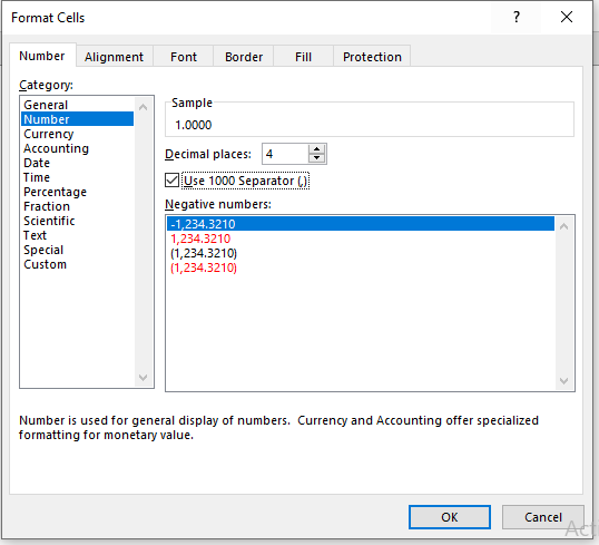
We can also select our numbers, right-click on any of the selected cells and then choose Format Cells:
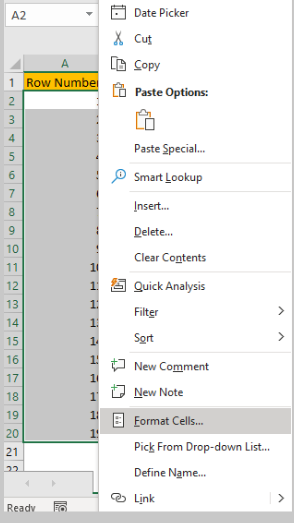
In both cases, we will be directed to the Format Cells pop-up window, from which we can choose various number formatting options:
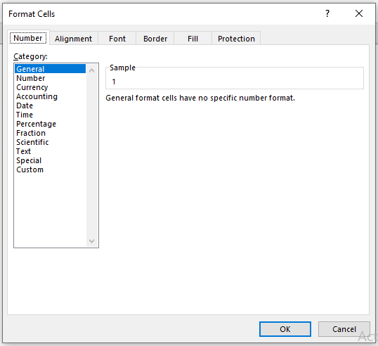
We can choose from various formatting options on the left side. We will click on Number and then choose 4 decimal places and select Use 1000 Separator:
When we click OK, we will see the change in the first column:
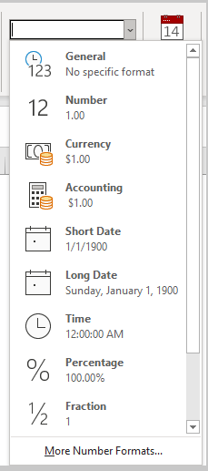
We can also get to these formatting options in a dropdown of our Home tab, and use predefined options that are at our disposal:
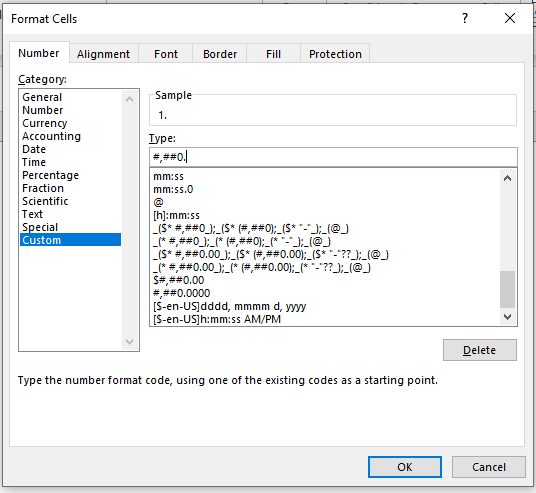
Custom Formatting Options
We can always define the formatting of our numbers ourselves. To do this, we will repeat the same steps to get to the formatting options, and then we will choose the last option- Custom:
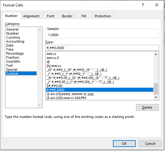
We will go beneath the Type option and delete the last four figures- zeroes. Our Type will now look like this:
And when we click OK, the results in our table will be the following:
