Highlight Rows Based on Drop Down List in Excel

As we work with Excel, we may want to highlight rows in a dataset based on the selection on a drop-down list in Excel. Highlighting rows based on a drop-down list selection in Excel can be a helpful way to organize and analyze data visually. In addition, by applying conditional formatting to the rows, you can quickly identify and compare rows that meet specific criteria.

This tutorial shows the process of highlighting rows based on user selection on drop-down lists in Excel.

How to Highlight Rows Based on Drop Down List in Excel

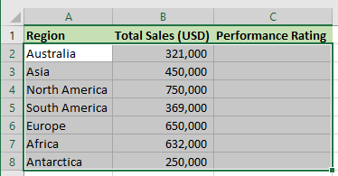
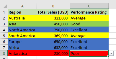
Suppose we have the following dataset on Sheet1 showing a particular technology company’s total annual regional sales.

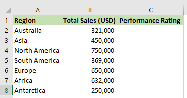
We want to create drop-down lists in column C that allow us to select specific performance ratings to highlight the rows that match the chosen performance ratings.

The conditional formatting would make it easy to see which regions have excellent, good, average, or poor performance ratings based on total sales.

We use the following steps:

Step #1: Create the Drop Down Lists

We create performance rating drop-down lists in the cell range C2:C8 using the steps below:

1. Create a list of performance ratings in cell range A1:A4 on Sheet2 and name the cell range “Performance Ratings.”

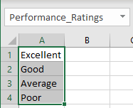
Note: You name the cell range by selecting it and typing the name in the Name box. The name must not have spaces.

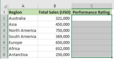
2. Select the cell range C2:C8 on the dataset.

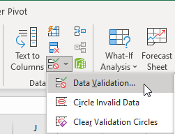
3. Click Data >> Data Tools >> Data Validation.

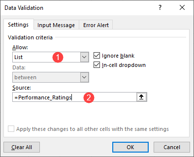
4. Do the following on the Settings tab of the Data Validation dialog box that appears:

• Open the Allow drop-down and choose List.
• Type the formula =Performance_Ratings on the Source box.
• Click OK.

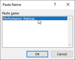
Note: Instead of typing the formula on the Source box, you can click on the Source box, press F3, select the name of the named cell range, and click OK to paste the name.

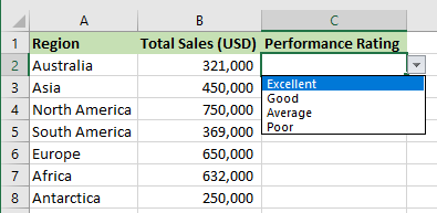
You can click the down arrow next to each cell in the cell range C2:C8 to test the drop-down lists created in the range:

Step #2: Apply Conditional Formatting

We want to apply conditional formatting to the dataset such that if the regional sales are:

• Above $500,000, we select Excelllet on the drop-down list and highlight the row in blue.
• Above $400,000 but less than $500,000, we choose Good on the drop-down list and highlight the row in green.
• Above $275,000 but less than $400,000, we select Average on the drop-down and highlight the row in yellow.
• Below $275,000, we choose Poor on the drop-down list and highlight the row in red.

To apply conditional formatting to the dataset based on selections on the drop-down lists, we do the following:

1. Select the entire dataset where we want to highlight rows based on drop-down list selection.

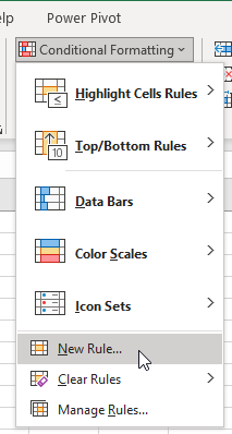
2. Click Home >> Styles >> Conditional Formatting >> New Rule.

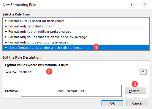
3. On the New Formatting Rule dialog box, select Use a formula to determine which cells to format on the Select a Rule Type box, enter the formula =$C2=”Excellent” on the Format values where this formula is true box, and click the Format button.

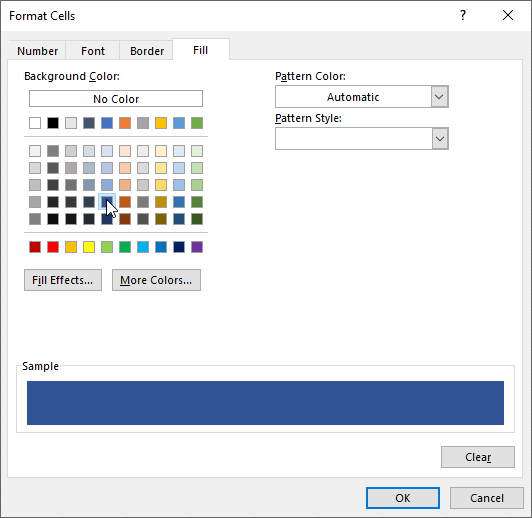
4. Open the Fill tab on the Format Cells dialog box, select the blue background color, and click OK..

5. Click OK on the New Formatting Rule dialog box.
6. Repeat steps 2-5 to apply the conditional formatting to the remaining drop-down values. Enter the formulas =$C2=”Good”,=$C2=”Average”, and =$C2=”Poor” for the Good, Average, and Poor performance rating rows. Additionally, specify the green, yellow, and red colors, respectively.

Step #3: Highlight Rows Based on Selections on Drop Down Lists

When you select an option from the dropdown list, the rows in the dataset that match that selection will be highlighted with the formatting you specified, as shown below:

Conclusion

This tutorial showed the process of highlighting rows based on drop-down lists in Excel. We hope you found the tutorial helpful.