Whenever you hear about highlighting in Excel, there is a good chance that you will be using Conditional Formatting. The options with formatting are limitless, as there is always a way to define the things that we want to be marked with a formula.
In the example below, we will show how to use Conditional Formatting to highlight a specific date, more precisely- today’s date.
Highlight the Current Date in Excel
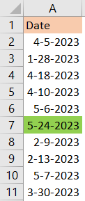
For our example, we will use the list of random dates ranging from the 1st of January of 2023 to today’s date (the date when this article was written is the 24th of May of 2023):
Looking at the table, we can clearly see that the date that we want to highlight is located in cell A7. To determine this with the formula, we will select our range, then go to Home >> Conditional Formatting >> New Rule:
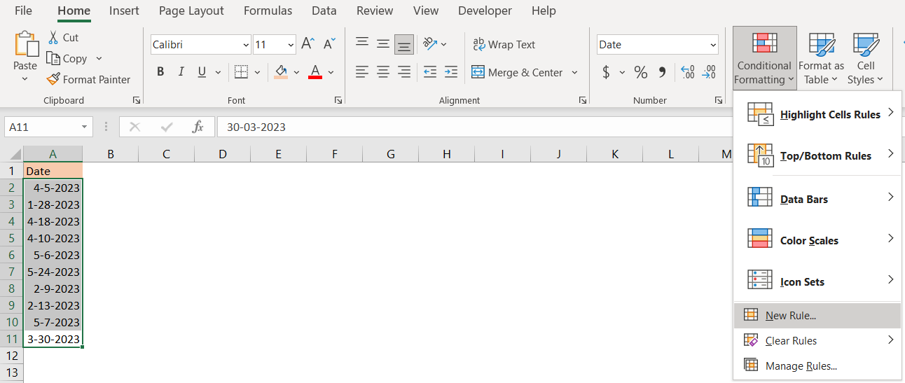
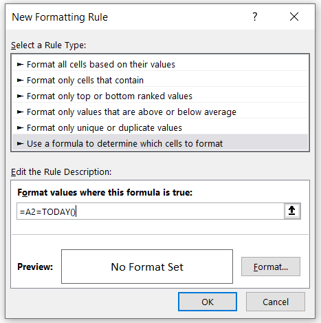
In the new window that appears, we will choose the last option available- Use a formula to determine which cells to format and insert the formula:
|
1 |
=A2=TODAY() |
Under the Format values where this formula is true input box:
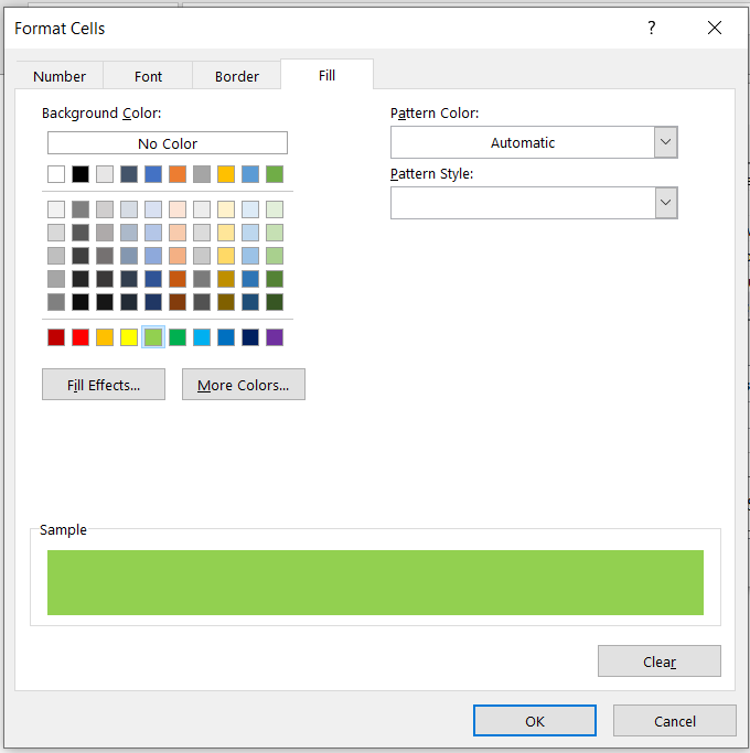
To actually highlight the cell that we want, we have to click on the Format button, then go to the Fill tab and choose a background color. We will use the green color for our example:
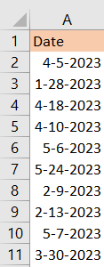
We will click OK, and will have our cell highlighted in the table: