Excel allows us to manipulate our data in every way possible. We can manipulate cells, rows, columns, ranges, and even the text in the cells as well.
In the example below, we will show you how to adjust your text in Excel, and even make it vertical, for the need of a report.
Make Text Vertical in Excel
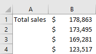
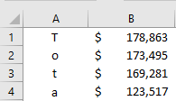
There are great tools in place with which we can manipulate our text. We will insert random sales numbers for four months:
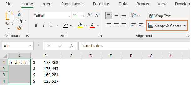
If we would like to make the text Total sales written vertical, and in line with numbers, the first thing we need to do is select the cell A1, then select the range A1:A4, and go to Home >> Alignment >> Merge & Center:
After taking this step, we need to select our cell one more time and go into the Alignment group in the Home tab one more time (you will notice that this is the group in which we can do a lot of text formatting) and click on the Orientation icon (as in the picture below):
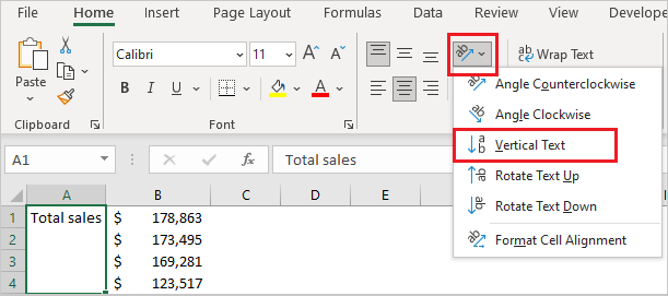
The orientation icon will give us some options, and among them, in third place, we will see the option for Vertical Text. When we click on it, our text will be written vertically:
It is noticeable that we cannot see the full two words now, the reason being that they take up too much space. We would have to expand the cells or resize the text to see it in full.
Vertical Text with WordArt
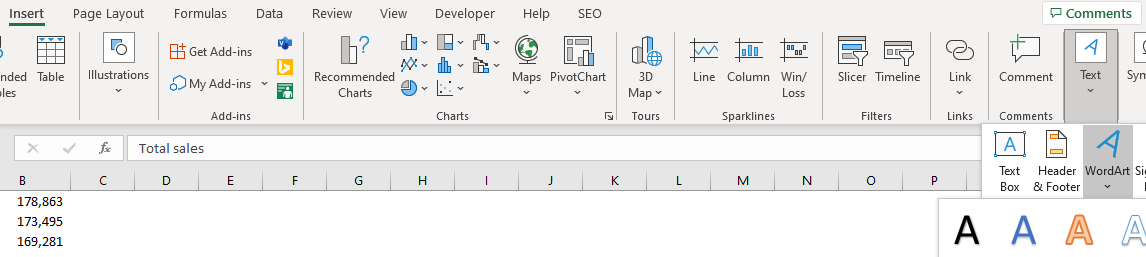
We can also use WordArt to make our text vertical. We go to the Insert tab, then go to Text >> WordArt:
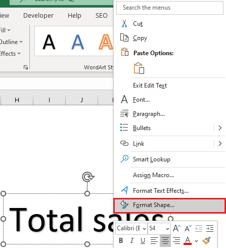
When we click on it, a text box will appear. We will write down “Total sales”, and then right-click on this text and choose Format Shape:
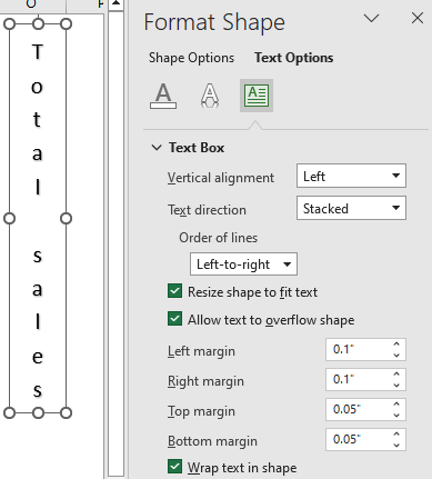
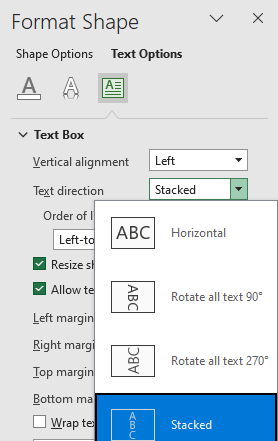
When we choose the Format Shape option, the formatting screen will appear on the right side of our screen. In the Format Shape option, we will choose Text Options and then choose Textbox:
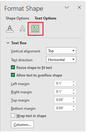
In this field, we will choose the Stacked for Text direction option:
When we click on this option, this is what our text looks like (the text was resized to fit the photo):