Increment Row Number in Excel

As you use Excel, there may be instances where you need to sequentially increase the row numbers. For example, assign individual identifiers or serial numbers to each row of data.

In Excel, there is no built-in feature to number rows automatically. Nevertheless, this tutorial presents seven methods to increase row numbers in Excel without manual input.

Method #1: Use Fill Series to Increment Row Numbers in Excel

We can use the “Fill Series” command to increment row numbers in Excel.

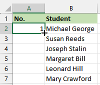
Suppose we have the following list of names:

We want to use the “Fill Series” command to number the rows in column A in the sequence 1, 2, 3, and so on.

We use the following steps:

1. Select cell A2 and enter “1,” the starting number.
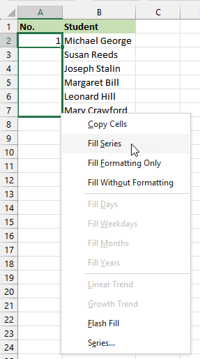
2. Select cell A2 containing the starting number, and hover the cursor over the fill handle in the bottom right corner of the cell until it changes to a small black cross sign (+) as shown below:

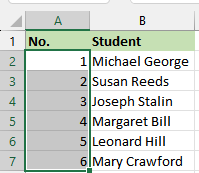
3. Press and hold down the right mouse button and drag to cell A7. Release the button and select “Fill Series” on the shortcut menu that appears:

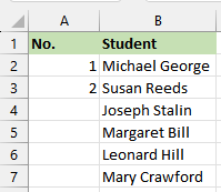
The list is numbered in the desired sequence as shown below:

Note: This method may become cumbersome when handling lengthy lists. In instances like these, we recommend utilizing the following method.

Method #2: Use Relative Referencing and AutoFill to Increment Row Numbers in Excel

We can use the combination of relative referencing and autofill to increment row numbers in Excel, as described in this method.

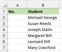
Assume we have the following list of names:

We want to use relative referencing and autofill to number the list in column A in the sequence 1, 2,3, and so on.

We use the below steps:

1. Select cell A2 and enter “1,” the starting number.
2. Select cell A3 and enter the following number, which is “2.”

3. Select cells A2 and A3 containing the starting number and the following number.

4. Double-click on the fill handle in cell A3. Excel will automatically fill the row numbers to the last row with data in the adjacent column.

Method #3: Add 1 to Number in Previous Cell to Increment Row Numbers in Excel

We can use a formula that adds 1 to the number in the previous cell to increment row numbers in Excel.

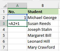
Suppose we have the following list of names:

We aim to create a sequence of numbers in column A, starting from 1 and increasing by 1 in each subsequent cell. To achieve this, we utilize a formula that adds 1 to the value in the cell immediately preceding it.

We use the following steps:

1. Enter the value 1 in cell A2.
2. Enter the following formula in cell A3:

3. Double-click the fill handle in cell A3 to copy the formula down the column. Excel automatically fills the row numbers to the last row with data in the adjacent column.

Method #4: Use the ROW Function to Increment Row Numbers in Excel

We can use the ROW function, which returns the row number of a reference to increment row numbers in Excel.

Suppose we have the following list of names:

We want to use the ROW function to number the rows in column A starting from cell A2 in the sequence 1, 2, 3, and so on.

We use the steps below:

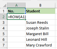
1. Select cell A2 and type in the following formula:

2. Double-click the fill handle in cell A2 to copy the formula down the column. Excel automatically fills the row numbers to the last row with data in the adjacent column.

Note: To have the numbers automatically added when you insert new rows of data, you can convert the data range into an Excel table. This will ensure that all the rows added to the end of the table are numbered accordingly.

Method #5: Use the SUBTOTAL Function to Increment Row Numbers in Excel

We can use the SUBTOTAL function, which returns a subtotal in a list to increment row numbers in Excel.

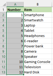
Let’s consider the following dataset:

We want to utilize the SUBTOTAL function to generate sequential numbers in column A in the order 1,2,3, and so on.

We use the below steps:

1. Select cell A2 and type in the following formula:

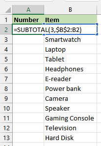
2. Double-click the fill handle in cell A2 to copy the formula down the column. Excel automatically fills the row numbers to the last row with data in the adjacent column.

Explanation of the Formula

The formula calculates a subtotal for a range of values.

Let’s break down the formula:

• The “SUBTOTAL” function calculates a subtotal for a given range based on a specified function number.
• “3” is the function number that represents the “Count” function. In this case, the formula counts the number of cells in the range that contain numeric values.
• “$B$2:B2” is the range of cells included in the calculation. “$B$2” represents an absolute reference to cell B2, and “B2” represents a relative reference. As the formula is filled down, the reference to cell B2 changes accordingly.

The first row displays the count for the range B2:B2; the second row displays the count for the range B2:B3, the third row for B2:B4, and so on.

Method #6: Use a Formula Combining the TEXT and ROW Functions to Increment Row Numbers in Excel

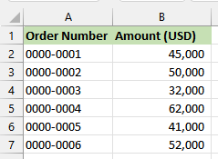
You can use a formula combining the TEXT and ROW functions to enter particular sequential number codes, such as purchase order numbers in a column, as shown below:

Let’s consider the following list:

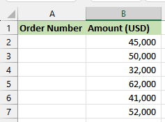
We want to enter sequential order numbers in column A in the format “0000-0000” using a formula combining the TEXT and ROW functions.

We use the below steps:

1. Select cell A2 and type in the following formula:

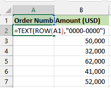
2. Double-click the fill handle in cell A2 to copy the formula down the column.

Explanation of the Formula

The formula converts the row number of cell A1 into a text string with a specific format.

Let’s break down the formula:

1. ROW(A1): The ROW function gets the row number of cell A1 which is 1. Although the list starts in row 2 because of the header, we use the cell reference A1 in the formula because we want the list to start with the number 1.

2. TEXT(value, format_text): The TEXT function formats a value based on a specified format. In this case, the formatted value is the row number returned by ROW(A1).

3. “0000-0000”: This is the format_text argument of the TEXT function. It specifies the desired format for the value. The format consists of eight digits divided by a hyphen. Each digit placeholder (0) represents a digit, and the hyphen (-) is a literal character.

The formula ensures that the resulting text string has eight digits including leading zeros, and a hyphen at the fourth position.

Method #7: Use a Formula Combining INT and ROW Functions to Increment Numbers Every X Rows in Excel

In the previous sections, we learned about Methods #1 and #2 to fill sequential numbers in a column. However, there may be situations where you need to fill a column with increment numbers every certain number of rows.

For example, you may want to fill the first four rows beginning with the number 1 (in this case, starting from row 2 because the dataset has a header), on the sixth row the number changes to 2, on the tenth row the number changes to 3, and so on as depicted in the below list:

We must use a formula combining the INT and ROW functions to achieve this numbering.

Suppose we have the following list of items:

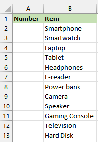
We want to use a formula combining the INT and ROW functions to fill column A with numbers in the sequence 1,1,1,1,2,2,2,2,…

We use the following steps:

1. Select cell A2 and type in the following formula:

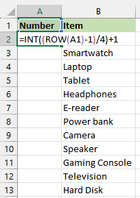
2. Drag or double-click the fill handle in cell A2 to copy the formula down the column.

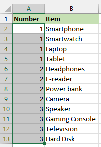
The first column is filled with sequential numbers that increase every four rows.

Explanation of the Formula

This formula generates a sequence of numbers that increments by the value 1 every four rows.

Here’s a breakdown of the formula:

1. ROW(A1): The ROW function returns the row number of the cell reference A1. Although our list begins in cell A2 because of the header, we use the reference A1 because we want the numbering to start from 1.

2. (ROW(A1)-1)/4: This subtracts 1 from the row number and divides it by 4. By subtracting 1, we ensure that the first row of the range produces a result of 0.

3. INT((ROW(A1)-1)/4): The INT function truncates the decimal portion of the division result, giving us the whole number quotient. For example, if the row number is 5, the result will be 1.

4. +1: Finally, we add 1 to the truncated result. This adjustment shifts the sequence by 1, making the first row of the range produce a result of 1.

Conclusion

This tutorial showed seven techniques for incrementing row numbers in Excel. We hope you found the tutorial helpful.