Many things in Excel are built-in, and they cannot be removed at all. Even if it is something that bothers us or we find it obsolete, it cannot be changed. One of these things is the row numbers being painted in blue.
In the example below, we will show how and why this occurs and how to deal with it.
Remove Blue Row Numbers in Excel
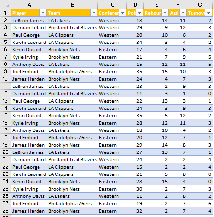
For the example, we will use the list of NBA players and their statistics from several nights:
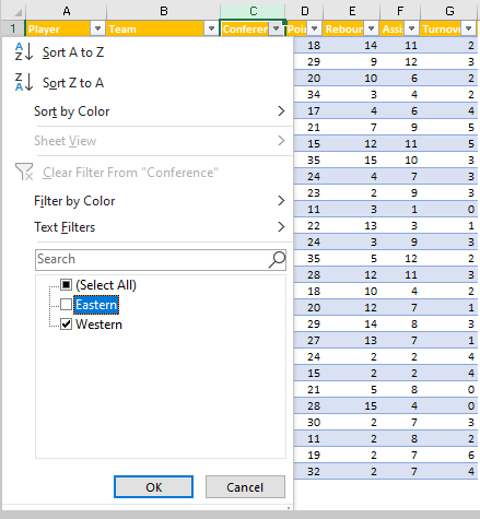
If we want to filter out only the players from the Western Conference, we will need to go to the dropdown arrow in cell C1, and then unselect the Eastern Conference as an option:
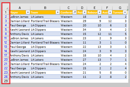
Once we click on it, we will have the following table of NBA players, along with the rows of the filtered players colored in blue:
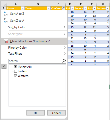
Now that we know the root cause of this issue (blue row numbers) we can easily resolve the issue. All we need to do is to remove the filters. We can go directly to the dropdown where we filtered the players from the Western Conference, and we will click “Clear Filter from Conference”:
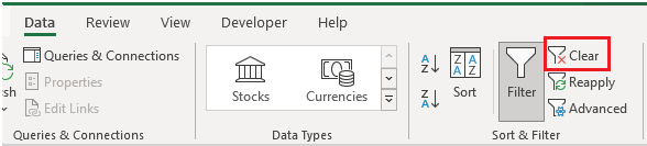
There is also another way to clear all the filters (if we had many, not just one). We need to go to Data tab >> Sort & Filter >> Clear:
This way, you will make sure that you remove the filter from the sheet entirely, and have the original table that we showed at the beginning.
This is also a certain time that blue row numbers are removed.