When speaking of the Pivot Tables, there are so many topics to be covered in Excel that you can never claim you covered everything.
We showed multiple things, such as how to create the Pivot Table, how to edit it, how to add a column to it, and finally, how to delete it.
In the example below, we will present the way to show the latest value in the Pivot Table.
Showing the Latest Value with Pivot Table
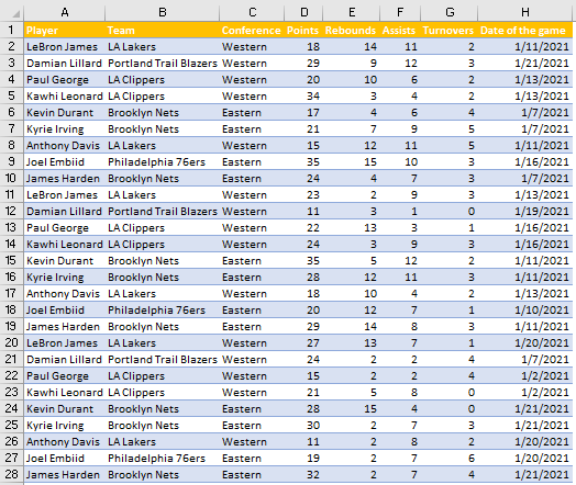
For our example, we will use the list of NBA players and their statistics from several nights. We will also add the dates when these games were played:

We will create the Pivot Table, put Player in Rows Field, Sum of Points, and Sum of Rebounds in Values Field:

To find out the latest game for every player, i.e. the last date when their games were played. To do this, we will simply add the Date of the game in the Values Field, then left-click on it there and choose Value Field Settings:

We will choose Max as an option for summarizing value fields by:

We do this because we want to get the latest data for every player. We already said that Excel is observing the dates as numbers, and the older dates have lower numbers, so when we choose the Max option, the highest number will appear, i.e. the latest numbers.
This is how our table looks like now:

From this point, we can filter out only the latest date. We will do that by clicking the dropdown right next to the Row Labels text, going to Value Filters, and then choosing Top 10:

From there, we will choose to show only 1 top value for Max of Date of the game:

We will have four values shown:

As there are four logs for this date (1/21/2021), which is a true result.
