Pivot Tables are useful because they can extract the data we have, summarize them, and give users a better visual presentation of it.
In the example below, we will show how to show the values from our Pivot Table in Rows.
Show Values in Rows in a Pivot Table
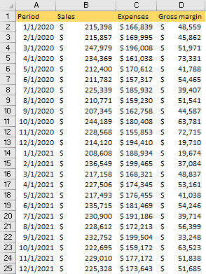
The first thing that we need to do is create the Pivot Table. We will do that from the data that shows sales, expenses, and gross margin for a certain company in a period from January 2020 to December 2021:
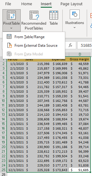
To create a Pivot Table, we need to select our table by clicking anywhere on our range and click CTRL + A, and then go to Insert >> Tables >> Pivot Table >> From Table/Range:
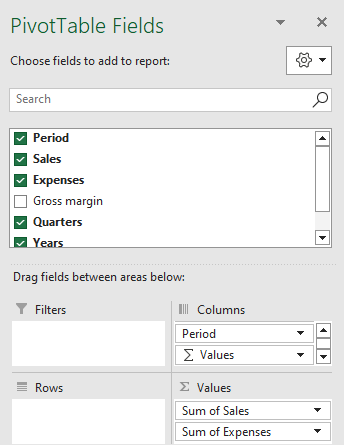
When the Pivot Table is created, we will insert Period data into the Columns field, and Sales and Expenses in Values fields:
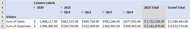
This is what our table looks like:
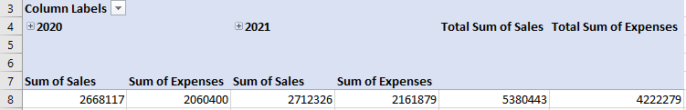
It is noticeable that we have the plus option in the dates, beneath the column labels. This is a great option that enables us to expand our data and show quarterly figures.
To see the data in rows, all we need to do is scroll down in Columns Field and then move Values to Rows:
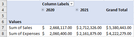
We will click on the plus sign next to the year 2021, and this is what we will end up with: