Excel Pivot Tables are one of the most important and useful things when it comes to extracting and presenting our data. The options in them are pretty straightforward, but some things that can be used might not be.
In the example below, we will show how to sort Pivot Table by grand total in Excel.
Sort Pivot Table by Grand Total
The first thing that we need to do is create our Pivot Table. As in many examples, we will use the data for NBA players and their statistics for several nights:

We will select the data by clicking anywhere in it and clicking CTRL + A, and then go to Insert >> Tables >> Pivot Table >> From Table/Range:

On the table that is created, we will put Player in Rows Field, and Rebounds, Points, and Assists in Values Field (in that particular order):

This is what our Pivot Table looks like:
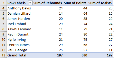
As seen, we have the rebounds in first place on our table. If we want to sort our table by Grand Totals, we would have to click right-click on any number in the Grand Total row, and then go to Sort and choose an option. In our case, we will click on Sort Smallest to Largest option:

When we do that, you will notice that the columns are now sorted from smallest to largest:
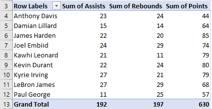
If we had our data in Column Field, rather than in Row Field, we would do the same thing, i.e. find the Grand Total and select any number in that column (rather than in row, which was our case). We also have multiple sorting options (as seen in the picture above) that we could use.