Cell highlighting can be a pretty useful tool when we work with data in Excel. We already explained a lot of possible scenarios and options for highlighting our data set.
In this text, we are going to show an example of how to highlight the same values in our range.
Highlight the Equal Cells with Rules
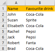
For the example, we are going to use the list of people and their favorite drinks.
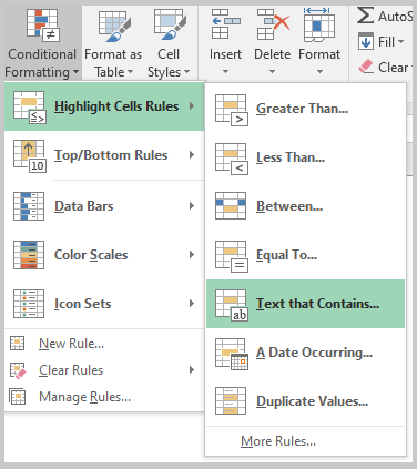
The easiest way to highlight only those rows with certain drinks, for example, Coca-Cola, would be to go to Home tab >> Styles >> Conditional Formatting >> Highlight Cells Rules >> Text that Contains:
In a window that appears, we will simply input the desired word. You will notice that we can see the preview of our changes in our rows even before we even click OK:
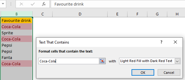
When we click OK, our table will be set and we will have all the rows in column B with Coca-Cola values highlighted.
Highlight the Equal Cells with Formula
There is another way to highlight our cells, and certainly, an easier one if we want to change the words that we want to highlight.
We will input the desired value that needs to be highlighted in cell E5. In our case, it is going to be the word „Pepsi“.
Next, we will select our range, and then go to the Home tab >> Styles >> Conditional Formatting >> Highlight Cells Rules >> More Rules.
On a window that appears, we will choose the final option- Use a formula to determine which cells to format:

We will input the following formula:
|
1 |
=B2=$E$5 |
We are referencing the first cell in our range (cell B2) and then we are checking if it is equal to the defined value in cell E5 (Pepsi). We locked this cell since it will not be changed. We will format the cells that are found to be colored in yellow.

After we click OK, our table will look like this:
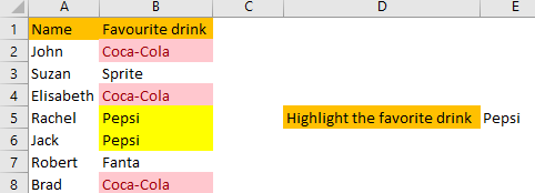
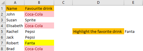
The beauty of our defined formula is that, if we want to highlight any other word, we simply need to change the value in cell E5. We will input the word “Fanta” in this cell, and our table will now look like this:
