Using a Dynamic Range With VLOOKUP in Excel

Sometimes we may need to use the VLOOKUP function when we expect additional rows or columns to be added to the data; therefore, the data range is dynamic. This tutorial shows how to use a dynamic range with VLOOKUP.

Use Excel Table

An Excel table is a feature that allows us to organize and manage data in a structured format. The Excel table automatically updates as new data is added to it. For example, when we use the Excel table as a table_array argument for the VLOOKUP function, the VLOOKUP automatically updates when new rows are added to the table. We do not need to adjust the range reference manually.

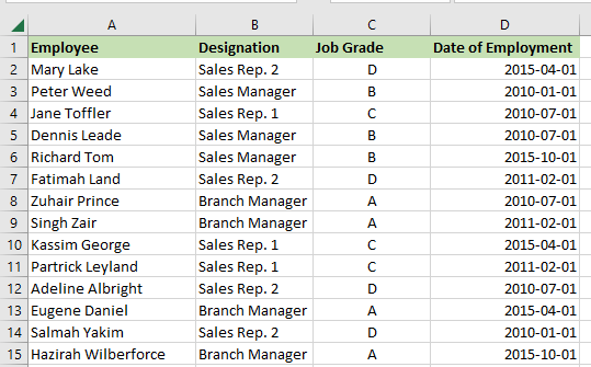
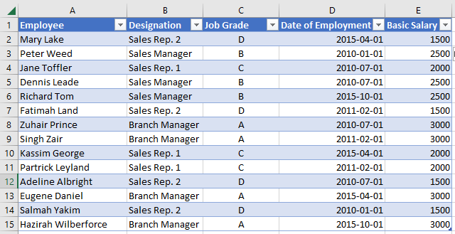
Suppose we have the following dataset on Sheet1 of our workbook. The dataset shows a particular company’s employee names, designations, job grades, and dates of employment :

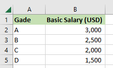
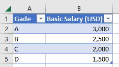
On Sheet2 of our workbook, we have the following dataset showing the company’s basic salaries for various job grades:

We want to use the VLOOKUP function to look up the employees’ basic salaries in the dataset on Sheet2 and display them in a column on Sheet1. Additionally, we want the VLOOKUP function to return the correct basic salary when new employee records are added to the employees’ dataset.

Step #1: Convert the Data Ranges to Tables

The first thing to do is to convert the data ranges on Sheet1 and Sheet2 to Excel tables.

We proceed as follows:

1. Open Sheet1 of the workbook.
2. Select any cell in the dataset and press Ctrl + T.

A moving ants border surrounds the dataset, and the Create Table dialog box appears. Notice that Excel has correctly guessed the dimensions of the dataset and the fact that it has headers. If the guess is incorrect, you can make the needed adjustments in the dialog box.

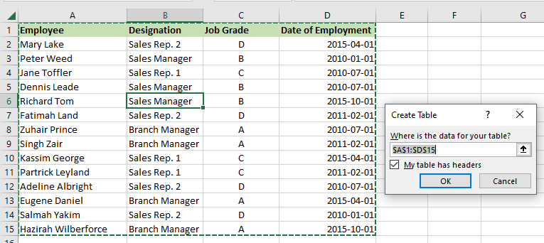
3. Click OK on the Create Table dialog box.

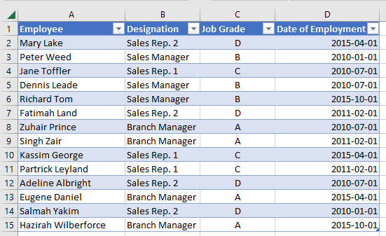
An Excel table is created immediately.

4. Convert the data range on Sheet2 to a table by selecting it and pressing Ctrl + T.

Step #2: Rename the Tables

The second step is to change the tables’ default names to meaningful ones using the below steps:

1. Open the workbook containing the tables we want to rename.
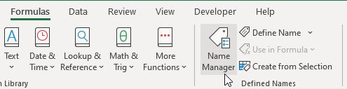
2. Click Formulas >> Defined Names >> Name Manager.

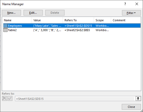
The Name Manager dialog box shows the two names used in the workbook.

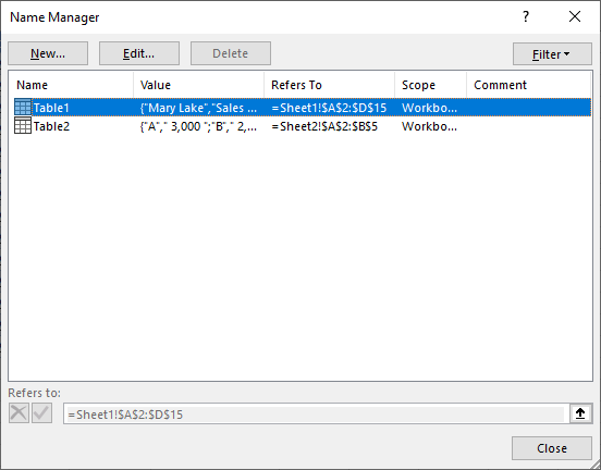
3. Select the first name, “Table1,” and click the Edit button on the dialog box.
4. In the Name box of the Edit Name dialog box that appears, type the name “Employees” and click the OK button.

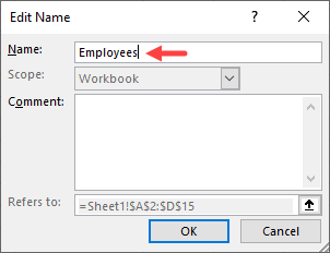
The first table is renamed Employees, and the new name appears in the Name Manager dialog box.

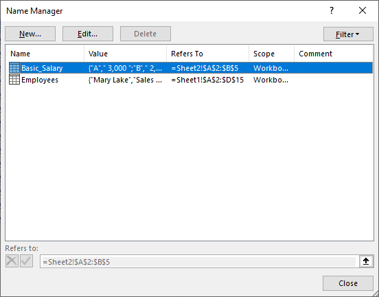
5. Select the second name, rename the second table “Basic_Salary,” and click the Close button at the bottom of the dialog box to close the dialog box. Notice that the name should not have a space character.

Step #3: Add a Column to the Employees Table

Select cell E1 on Sheet2 and type in the column header, “Basic Salary.”

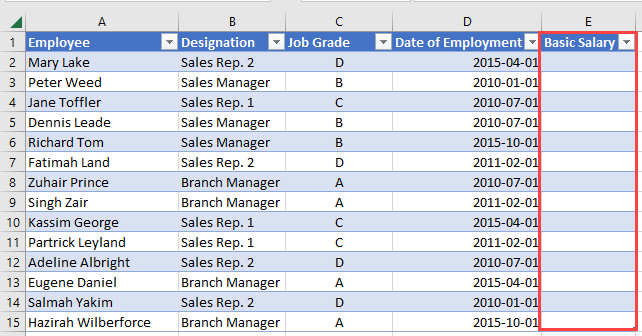
Notice that the table expands to accommodate the new column.

Step #4: Add a VLOOKUP Formula to the New Column

We need to add a VLOOKUP formula to the Basic Salary column in the Employees table.

We use the following steps:

1. Select cell E2 in the Employees table and type in the following formula:

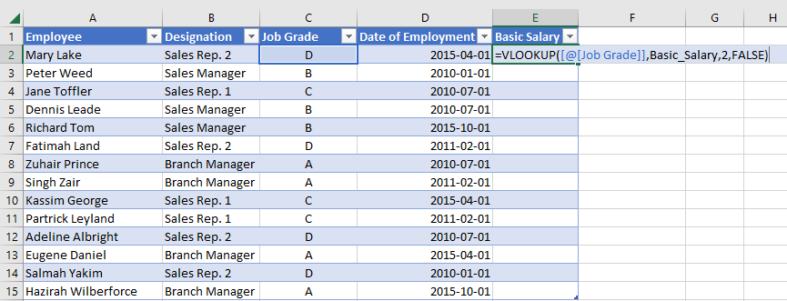
2. Press Enter.

The basic salary for each employee is filled in.

Explanation of the formula

We can interpret this formula to say, “Lookup the exact match of the value on this row in the Job Grade column in the leftmost column of the Basic_Salary table and return the value in the second column.”

Step #5: Test the VLOOKUP Formula

Suppose the company hires a new branch manager called “Bill George” on January 20, 2022. The new hires’ job grade is A.

Let’s add the new employee’s record to the Employees’ table.

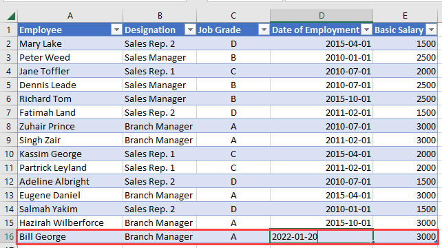
Notice that as we entered the new employee’s job grade in cell C16, the VLOOKUP formula suddenly entered his basic salary in cell E16.

Conclusion

This tutorial showed using a real-life example that to use a dynamic range with VLOOKUP in Excel, we have to create a named range that updates automatically as new data is added to the table. By using a named range, the VLOOKUP automatically updates when new data is added to the table, and there is no need to adjust the range reference manually.

We hope you found the tutorial helpful.