Excel uses round brackets ( ), square brackets [ ], and curly brackets { } for different purposes.
It is important to know when and to use the three different types of brackets used in Excel.
In this tutorial, we will look at each type of bracket and its uses in Excel.
Round Brackets or Parentheses ( )
In Excel Formulas
The round brackets or parentheses are mostly used within Excel formulas.
They are used within formulas to instruct Excel to first evaluate that part of the formula that is within the brackets. Whatever is in the bracket will be evaluated first.
For example, 10 + 2 *5 will result in 20 because Excel follows the conventional order of operations where multiplication precedes addition. Excel will first multiply 2 and 5 to get 10 and then add the 10 to 10 to get 20.
However, if we use the round brackets as in (10 + 2) * 5, the answer will be 60 because Excel evaluates what is in the round brackets first. In this case, Excel adds 10 to 2 to get 12 and then multiplies the 12 by 5 to get 60.
Excel must evaluate what is in the brackets first.
Within Excel Functions
The round brackets are also used within the Excel functions.
Functions are Excel’s inbuilt formulas such as the VLOOKUP and INDEX functions.
The round brackets In addition to the equal sign (=) that always precedes a formula in Excel are a standard feature of Excel functions. For example, in the formula =SUM(A1:A3) the SUM function encloses the range A1:A3 in brackets.
Every opening bracket must have a closing bracket otherwise Excel will generate an error. If we are doing a simple calculation and we fail to add a closing bracket, Excel may add a bracket for us automatically. Otherwise, it may also allow us to accept the correction it suggests or ask us to correct the error ourselves.
In Custom Number Formatting
Round brackets can be used in custom number formatting to display negative values in parentheses.
Excel does not come with a predefined format for displaying negative values in parentheses. If we prefer displaying negative values in parentheses or brackets, we have to create a custom number format.
One advantage of displaying negative values in parentheses is that they are easy to spot especially in large datasets.
We will use the following dataset of negative values to explain how to create a custom number format for displaying negative values in parentheses:
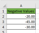
- First, select the range A2:A4.
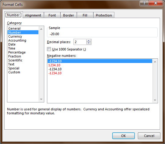
- Press the keyboard shortcut Ctrl + 1 to launch the Format Cells dialog box:
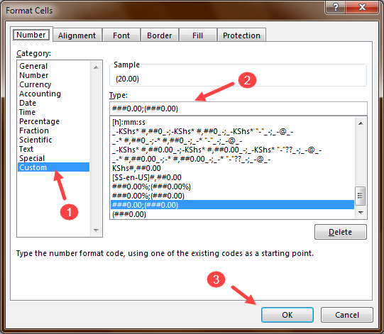
- Under the Category Area select Custom and in the Type box type in the number format ###0.00;(###0.00) and then click OK:
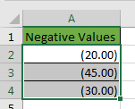
The negative values are displayed within parentheses:
Used in Adding further information within Text
The round brackets can be used to enclose additional information within the text. For example in an instruction written in an Excel sheet below the additional information is captured in parentheses:

Square Brackets [ ]
Excel uses square brackets [ ] to show references to external workbooks and also for structured references in Excel tables.
To Show References to External Workbooks
For example, the formula =[Sales.xlsx]Sheet1!$B$10 instructs Excel to look for the value in Cell B10 in Sheet1 in an external workbook called Sales.
The best way to ensure that Excel refers to the correct reference in an external workbook is to use the keyboard or mouse to select the correct range in the external workbook rather than typing in a range reference.
For Structured References in Excel Tables
The square brackets are also used for structured references in Excel named tables.
The named tables are created by clicking Insert >> Tables >> Table on the Excel Ribbon or by pressing the keyboard shortcut Ctrl + T. Excel allocates a name to the table and each column header.
When we add formulas to the named table and select cell references, the table name, and the column names appear automatically so that we do not need to enter them manually. The combination of the table name and column names is called a structured reference.
The structured references make it easy to refer to data in the named tables.
For example in a table named AnnualSales with a column named First Quarter Sales occupying cells D2:D20, Excel will use the structured reference =SUM(AnnualSales[First Quarter Sales]) to generate the total sales for the first quarter of the year instead of the explicit cell references =SUM (D2:D20).
Curly Brackets { }
Used in Array Formulas
The curly brackets are used in the specialized formulas called array formulas. These are formulas that can perform multiple calculations on one or more items in an array.
If you are not using Excel 365, the curly brackets are added by pressing Ctrl + Shift + Enter to accept the formula.
For example, if we press Ctrl + Shift + Enter after typing in the formula =D2*D3 in a cell, the formula will turn into {= D2*D3}.
Used to Group Information
The curly brackets can also be used as shapes to group information together.
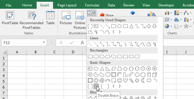
To insert the left curly bracket click Insert >> Illustrations >> Shapes >> Left Brace on the Excel Ribbon:

To insert the right curly bracket click Insert >> Illustrations >> Shapes >> Right Brace on the Excel Ribbon.
If we want to insert both the left and right brace at once, we should click Insert >> Illustrations >> Shapes >> Double Brace on the Excel Ribbon:
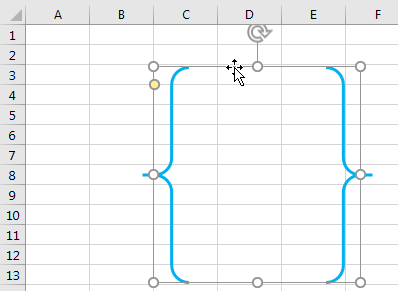
The brackets that are inserted as shapes can be customized as we like. For example, we can drag the border to change its size and location. We can even change their color and other effects:
Conclusion
In this tutorial, we looked at the three different types of brackets used in Excel and their uses. We also looked at when and how to use them.
Excel uses round brackets ( ), square brackets [ ], and curly brackets { } for different purposes.
The round brackets are used within Excel formulas and functions, custom number formatting, and to enclose additional information within the text.
The square brackets are used in formulas to show references to external workbooks and in the structured references in Excel tables.
The curly brackets are used in array formulas, grouping information together.
