How to Change Month from Text to Number in Excel

Excel has many helpful tips and tricks that people are usually not aware of. One of them is to convert the name of the months into numbers.

Although you might think that this issue could be formatting-related, it is actually a matter of using the correct formula. We will show that in the example below.

Change Months from Text to Numbers

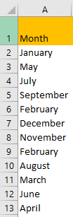
For our example, we will use the table with months that are not ordered chronologically:

Now, we will put the following formula into cell B2:

To explain how this works, we have to explain formulas separately:

DATEVALUE is a function that returns a serial number from a date that is in text format.

We have to use the „&“ symbol and any number to make Excel convert the text into a number.

MONTH function returns the value of the month from 1 to 12.

So, with our formula, we make Excel recognize the number of our month and then return this number to our cell.

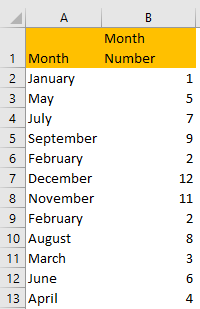
When we drag the formula to the end of our range, our table will look like this:

You will notice that this formula returned the proper values for every month in our table.

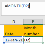
If we had the whole date, to find out the serial number of the date, we can use the MONTH formula as a standalone one, like in the example below: