All of the formulas in Excel are great on their own. Better yet, these formulas are even better when combined.
In the example below, we will show how to combine some of them: MATCH, INDEX, and OFFSET.
Combining MATCH, INDEX, and OFFSET
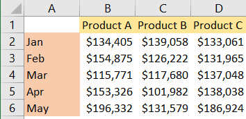
For our example, we will use the list of different products that were sold in different periods (months). This will what our table will look like:
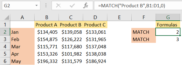
We will first show the MATCH formula and then go from that. We will write our formula in column G, cells G2 and G3. Our formulas will be:
|
1 2 |
=MATCH("Product B",B1:D1,0) =MATCH("Mar",A2:A6,0) |
And the results for these formulas will be 2 (position of Product B in the list of products), and 3 (position of the month of March in the list of months):
Now, the MATCH formula is pretty obvious. It finds us the relative position of the lookup value in our array.
For the next thing, we will insert the INDEX and MATCH formulas together:
|
1 |
=INDEX(B2:D6,G3,G2) |
In the table, it looks like this:
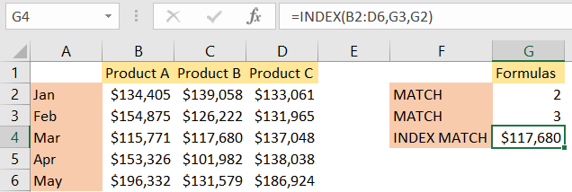
As seen in the formula, our array is B2:D6, our row number will be the number 3 (the row that corresponds to the month of March), and the column number will be number 2 (the column of Product B).
We use INDEX to get the number $117,680.
To use OFFSET in combination with these two formulas, we will write down the following formula:
|
1 |
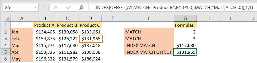
=INDEX(OFFSET(A1,MATCH("Product B",B1:D1,0),MATCH("Mar",A2:A6,0)),1,1) |
This formula will return number $131,965, located in cell D3:
But how did we get here? First, we have to look at MATCH formulas. First one: MATCH(“Product B”, B1:D1,0) searches for Product B in the first row, and it will find it in cell C1, or position number 2. Second MATCH function: MATCH(“Mar”, A2:A6,0) searches for the month of March in the list of our months, and it is located in position number 3.
OFFSET function has three mandatory parameters: reference, rows, and columns, and two optional (height and weight). We first declare our reference cell and then define the number of rows and columns that we will offset from this original cell.
OFFSET function will return a range that starts from cell A1 (OFFSET(A1, part of the formula) and shifts from this cell by the number of rows and columns that we defined in our MATCH functions. First MATCH is the offset for rows from our defined cell, so we will move for 2 rows from our number. The second MATCH is the offset for columns, and we will move for 3 columns from column A.
In the end, INDEX(range,1,1) retrieves the value at the intersection of the range obtained from OFFSET. The 1s as arguments refer to the first row and first column of the range.