Excel VLOOKUP and MID for Data Analysis

Excel formulas are made in a way that complicated things can seem easy. There is always an option to combine the formulas to extract the data and to get valuable information from our data set.

In the example below, we will show how to combine VLOOKUP and MID formulas to get the results we want.

Explaining Vlookup and Mid Functions

To show how these two functions operate together, we will first inspect each of these formulas separately:

1. VLOOKUP formula searches for a value in the first column of a certain range (in most cases table) and then it returns a corresponding value from that column in the same row. The syntax of VLOOKUP is:

• lookup_value: The value we are searching for.
• table_array: The range of cells where we are performing the search.
• col_index_num: The column number (1-based index) from which we want to retrieve the result.
• range_lookup: Optional. If TRUE (or omitted), an approximate match is performed; if FALSE, an exact match is performed.

1. A MID function is used to extract a specific number of characters from a text string, starting at a specified position. Its basic syntax is:

• text: The text string from which we want to extract characters.
• start_num: The position of the first character we want to extract.
• num_chars: The number of characters that we are extracting.

Combining VLOOKUP and MID formula

For our example, we will use the list of products, their codes, and sales records. Products will be Product A, B, and C:

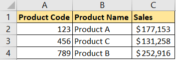
Now, let’s suppose that the product code originally consisted of both numbers and letters and that we have one original code looking like this:

ABC123ABC and GHI789GHI

We will store it in cells E2 and E3. Now there is a clear pattern here in which the shortened codes (number) begin from the fourth character in this extended code.

Now, if we want to find the sales of the original codes, we can do it with VLOOKUP and MID. In cell F2 we will insert the following formula:

But we will be returned with an error:

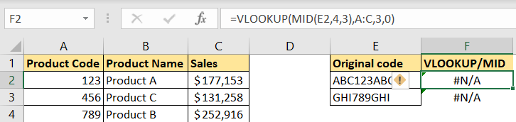
This formula uses the result in our MID formula as a lookup value. MID formula retrieves three numbers from our designated cell starting from the fourth character. The table array for our VLOOKUP are columns A:C, and we are searching for the sales values, located in the third column.

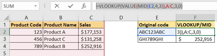
But why do we get an error? The reason why this happens is that the MID function is a string function that always returns TEXT format. We are obviously looking for a number in our case. To change this, we need to add the VALUE formula, which has only one parameter – TEXT (this formula basically converts text to number). Our formula will now be:

And we will get the expected result:

Now, this example is extremely simplified, but it shows a combination of formulas that can be used in more complex situations and datasets.