Excel VLOOKUP With Multiple Results

Although VLOOKUP is a very useful formula and can help us get the results we want with success and easier, certain shortcomings are worth mentioning.

One of those things is to retrieve multiple results with VLOOKUP. However, there are some workarounds to resolve even this issue.

Using the FILTER function

For our example, we will use the simple table of sales data, with the names of salespersons that achieved those sales:

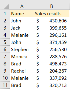
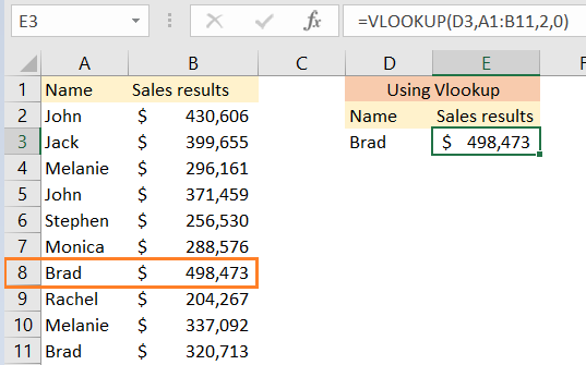
You will notice that some names, such as Brad, are found multiple times on our table. If we would go and use a VLOOKUP to extract only the data for Brad from our table, we would end up only with the sales results of the first instance of the name (row number 8):

To get the result for the second Brad, we cannot use VLOOKUP, at least not with the current state of our table. To get the results for both persons named Brad, we can use the FILTER formula. This is a relatively new formula that is available in Excel Online or Microsoft 365 version.

It has three parameters, out of which two are mandatory, and the last one is optional. The first parameter is the array, and it represents the range that we want to filter. The second one is include, and it stores our filter criteria. The third one is the if_empty parameter, which we use to display a value of our choosing if the formula does not retrieve anything.

In our example, the array will be column B (sales results), and include will search for all the values Brad in column A.

Having in mind that we will insert the word Brad in cell D6, this will be our formula:

And the results will be displayed in sequential order, one after the other:

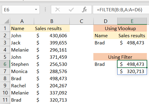
The fact that the cell borders are blue goes to show that this is a built-in function in Excel.

VLOOKUP With Multiple Results

There is a workaround for using VLOOKUP to achieve the same results that we had with the FILTER formula above. To achieve this, we first need to insert the helper’s column, to give a unique identifier for every name in our table.

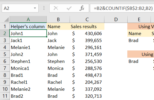
We will add a column in front of column A, and insert the following formula in cell A2:

This formula will check if the value in column B exists already. If it does, a number will be added to it. When we drag this formula till the end of our table, this will be the result:

At this point, we can simply use the unique identifier to retrieve our results, but that would not help us a lot. Instead of that, we will change the lookup_value, and this will be a lookup_value for our VLOOKUP formula:

In cell H3, we will put the name of the persons that we want to retrieve the results for. We concatenate this result with the ROW formula, and we will use the rows located in column A. Our table array will be range A2:C11. As a final result, this will be a formula that we will insert in cell I3:

In the previous versions of Excel, you would need to press CTRL + SHIFT + ENTER before inserting the formula. In the online version of Excel and Office 365, we do not need to do this, as the formula will be laid out to us:

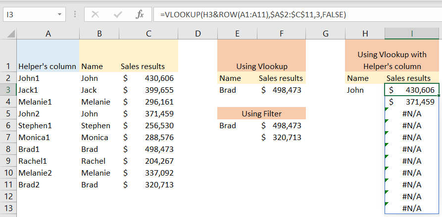
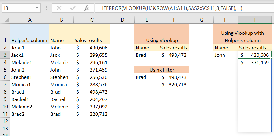
You will notice that we have a lot of #N/A results. To get rid of these, we will add IFERROR at the beginning of the formula, so it will be:

And our results will look much better: