In Excel, we can use the VLOOKUP function to find a table’s column index number of a specific value.
This tutorial shows how to use the Excel VLOOKUP function to find the column index of a particular value in a table array.
Find The Column Index Number Using VLOOKUP in Excel
VLOOKUP is an Excel function that allows you to look up a value in a table and return a corresponding value from a specified column.
Syntax of the VLOOKUP Function
The syntax of the VLOOKUP function is as follows:
=VLOOKUP(lookup_value, table_array, col_index_num, [range_lookup])
Where:
- lookup_value is the value you want to look up.
- table_array is the range containing the lookup value.
- col_index_num is the column number in the table_array that contains the value you want to return.
- range_lookup is an optional argument that specifies whether you want an exact or approximate match for lookup_value. If range_lookup is TRUE or omitted, an approximate match is returned; if range_lookup is FALSE, an exact match is returned.
Find the Column Index Number
One of the required arguments of the VLOOKUP function is the column index number, which specifies the column from which the function should return the corresponding value.
Using the VLOOKUP function to find the column index number is applicable when you have a table with many columns and need to perform a lookup based on a specific column header. Instead of manually counting the number of columns to determine the column index number, you can use the VLOOKUP function to automate the process.
Let’s consider the following example dataset showing the prices of branded electronic items.
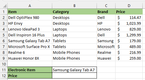
We want to use the VLOOKUP function to find the index number of the column containing the price of the Samsung Galaxy Tab A7 tablet.
Note: The example dataset is small; therefore, we can quickly tell that the price column is number 4 in the table array by manually counting the columns.
However, you can have a table with many columns, making it inconvenient or challenging to determine the target column index number manually. Therefore, you can use the VLOOKUP function to determine the column index number automatically.
We use the following steps to find the price column index number using the VLOOKUP function:
- Select cell B2 and type in the following formula:
|
1 |
=VLOOKUP(B11,A2:D9,COLUMN(D1)-COLUMN(A1)+1,FALSE) |
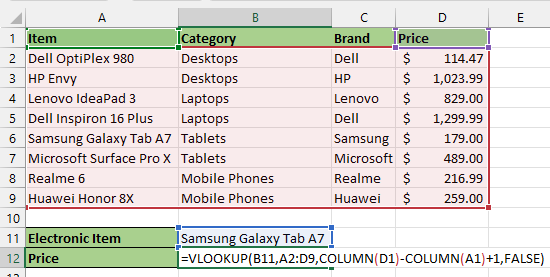
- Press Enter.
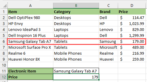
The formula returns the value 179, which is the Samsung Galaxy Tab A7 tablet price contained in cell D6 in column 4 of the dataset.
Explanation of the formula
|
1 |
=VLOOKUP(B11,A2:D9,COLUMN(D1)-COLUMN(A1)+1,FALSE) |
This formula’s look value is “Samsung Galaxy Tab A7” in cell B11. The table array is the cell range A2:D9.
The COLUMN(D1)-COLUMN(A1)+1 part of the formula uses the COLUMN function, which returns the column number of a reference to calculate the column index of the price column:
- COLUMN(D1) Returns the value 4, which is the column number of the price column from which we want to return the Samsung Galaxy Tab A7 price.
- COLUMN(A1) Returns the value 1, the column number of the column containing the lookup value.
The value 1, the column number of the column containing the lookup value, is subtracted from 4, the column number of the price column. Then the difference is increased by one, and the result is 4, the column index number of the column containing the price of Samsung Galaxy Tab A7, the lookup value.
Note: The range_lookup optional argument is set to FALSE because we want an exact match for the look-up up value.
Conclusion
This tutorial explained how to use the VLOOKUP function in Excel to find the column index of a particular value in a table array. We hope you found the tutorial helpful.