Find Missing Values Between Two Columns in Excel

When dealing with data in Excel, you need to keep in mind that, if you have a certain assignment, there is usually a way to do it in an easier way.

We will show that in the example below, where we will show how to find missing values between two columns.

Find Missing Values Between Two Columns

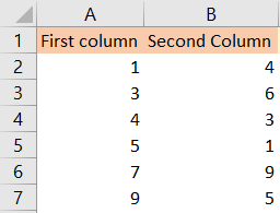
To find the differences between the two columns, we first need to have actual columns for comparison. In the two columns that we will create, we will insert numbers ranging from 1 to 10 (in both columns):

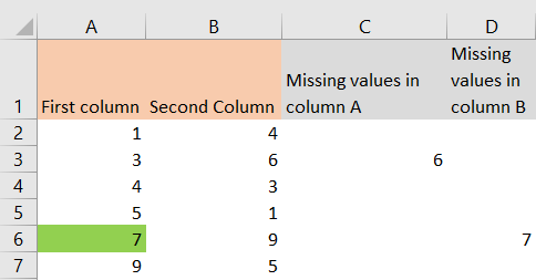
If we would go and manually look for the things that we have in the first column, but do not have in the second one, we would come to the conclusion that the number 7 (cell A6) can be found only in one column- column A. This goes both ways, as we have number 6 located in column B (cell B3) and we do not have this number at all in column A.

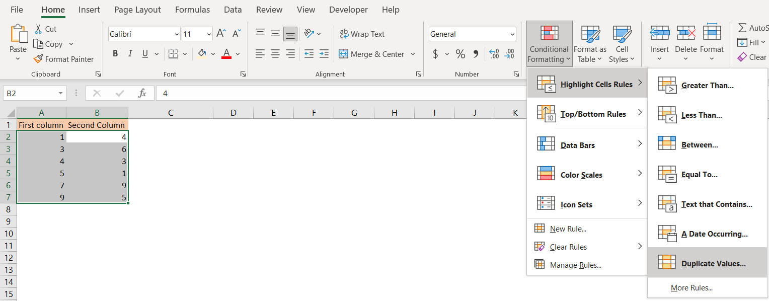
We can easily visually present this by selecting the data, and then going to Home >> Conditional Formatting >> Highlight Cells Rules >> Duplicate Values:

When we click on this, we will be presented with a dialog box that would let us highlight all the duplicated values with the color of our choosing. We will choose the generic option (light red fill with dark red text) and click OK:

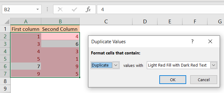
Number 7 in column A and number 6 in column B will remain in white, which clearly indicates that these numbers are the ones that are missing.

However, there is a huge downside to this approach. If we had the number 7 in the first column, this number would not appear as the odd one, as it would have its match.

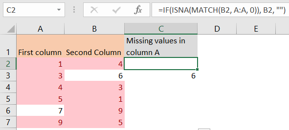
To find the missing values, we will use a formula. We will insert this formula in column C:

This formula checks if the value in cell B2 exists in column A. If this value does not exist, it will show us the value from cell B2. Otherwise, we will end up with an empty string.

When we drag and drop our formula till the end of our table, this will be our result:

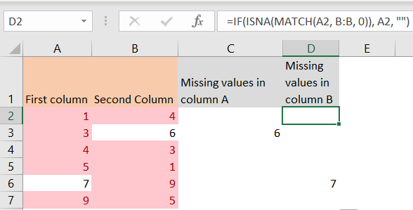
To check the missing values in column B, we will use the same formula, with the difference being that we are checking values from the B column in column A. This will be the formula in cell D2:

And our end result will be:

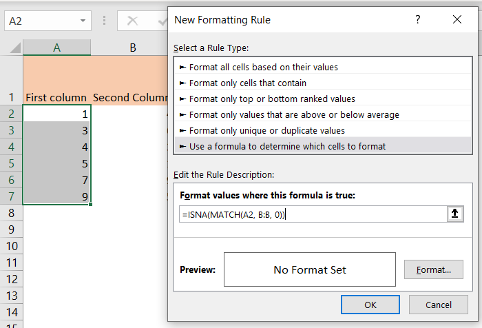
This formula can also be used in Conditional Formatting to highlight the proper numbers that are missing. To achieve this, we will select the data in column A, then go to Home >> Styles >> Conditional Formatting >> New Rule. Under New Rule, we will choose the last option available >> Use a formula to determine which cells to format, and will insert the following formula in Format values where this formula is a true section:

We will click on the Format and choose a Fill tab and then select any color for the background (in our case, the green one), and click OK:

When we click OK, we will have the desired results: