Finding the Maximum Value With HLOOKUP

To find the maximum value in an Excel table with HLOOKUP, you can combine the MAX function – which returns the largest value in a group of values – and HLOOKUP.

About HLOOKUP

The HLOOKUP function searches for a specific value in the top row of a table or array of values and obtains a value in the same column from the row of your choice. The term “H” in HLOOKUP refers to “Horizontal.”

Apply the HLOOKUP function if you need to search for specific data in a table where comparison values are located in a row at the top and you want to look down a particular number of rows.

The Syntax of HLOOKUP

The syntax of the HLOOKUP function is as follows:

HLOOKUP(lookup_value, table_array, row_index_num, [range_lookup])

Here’s the explanation of the arguments:

• Lookup_value This is required, and it refers to the value to be searched in the first row of the table.
• Table_array This is required and refers to a table of information in which data is looked up.
• Row_index_num This is required, and it indicates the row number in table_array from which the matching value will be returned.
• Range_lookup This is an optional and logical value that specifies whether you want to find an exact match or an approximate match. If TRUE is omitted, an approximate match is returned, and if FALSE, an exact match is returned.

How to Find the Maximum Value Using HLOOKUP

To find the maximum value in Excel using the HLOOKUP function, you would need to follow these steps:

Step #1: Set Up the Data

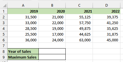
Ensure that your data is organized in a tabular format, with row headers in the first row and values in the subsequent rows, as in the example below:

Step #2: Enter Formula to Identify the Maximum Value

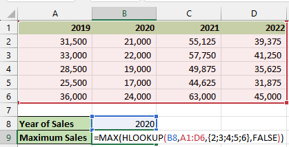
Assume we want to find out the maximum sales of 2020 in the example dataset shown in the previous step. We use the following steps:

1. Enter the lookup value “2020” in cell B8.
2. Type the following formula in cell B9.

3. Press Enter.

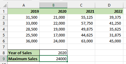
The maximum sales value for 2020 is displayed in cell B9 as shown below:

Explanation of the Formula

In this formula, the HLOOKUP function searches for the value in cell B8 within the range A1:D6. It then retrieves values from rows 2, 3, 4, 5, and 6 based on the exact match found. Finally, the MAX function returns the maximum value from those retrieved values.

Tip

Consider using the XLOOKUP function, which is an upgraded version of HLOOKUP. XLOOKUP can be used in any direction and provides exact matches by default, making it more user-friendly and convenient than HLOOKUP.

Conclusion

This tutorial described finding the maximum value in an Excel dataset with HLOOKUP. We hope you found the tutorial helpful.