Get Cell Value From Address in Excel

When working with Excel, in certain instances, you would like to know the value of your cell based on its location. To do this, you can immediately assume that we will have to use the ADDRESS function. You would be right.

We will show how to do this in the example below.

Using Address Function

For our example, we will use the table with NBA players, and their statistical data from one night of basketball, which includes points, rebounds, assists, and turnovers:

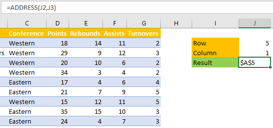
In column I, we will add the cells for the Row and Column. Next to it, we will add the row and number column (5 and 1) and then insert the ADDRESS function using these numbers. This will be our function:

And the results are:

ADDRESS function does exactly what we could see above- it returns the cell address with the given row and column.

Combining Indirect and Address to Get Cell Value

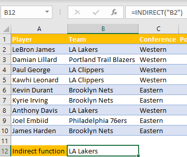
As seen, the ADDRESS function will not return the actual value from our cell, just the reference. To achieve this, we need to add the INDIRECT function as well. This function can return a valid reference from our text string. As seen in the example below, cell B12 (where we will put this formula) returns the value “LA Lakers”.

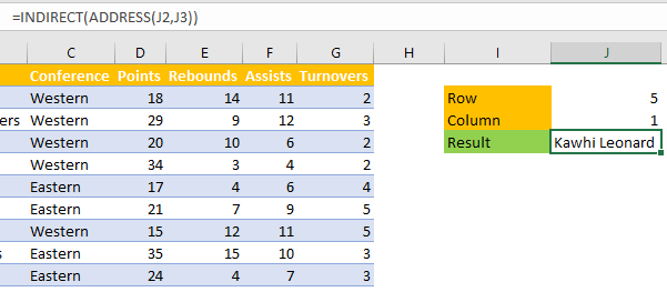
All we need to do now is combine these two functions that we discussed. We will do that in cell J4, where we had the results of the ADDRESS function before. Our formula will be as follows:

Which will give us the expected results: