A lot of user experience issues and problems in Excel are related to formula issues. One of these issues is having the #N/A values in your range, which can be quite disturbing. These values mean that there is no value available.
We will show a couple of formulas that can help you to sum or to find the average of your range even if you have certain values that cannot be found.
Ignore #N/A Values with Excel Formulas
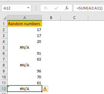
The first thing that we need to do is create a range with some values that cannot be found:
If we would go on and input the following formula:
|
1 |
=SUM(A2:A11) |
To sum all the values, we would end up with the results shown in the picture below:

This is pretty much expected. We need to tweak this formula a little bit, and there are a couple of options. We will type them in a range C2:C4:
|
1 2 3 4 |
=SUMIF(A1:A11,"<>#N/A") =SUM(IFNA(A2:A11, "")) =SUM(IFERROR(A2:A11,"")) |
All of these formulas listed above will get us the same result:
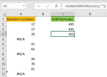
Which is exactly the result that we want and would have expected.
If we want to find out the average of our range, we would resort to the similar formulas:
|
1 2 3 |
=AVERAGE(IFERROR(A2:A11,"")) =AVERAGE(IFNA(A2:A11, "")) |
We will input these formulas in cells D2 and D3, and get the following results:
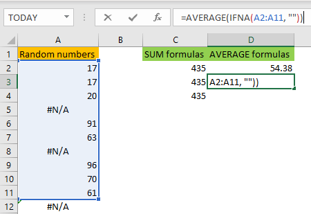
Personally, the best option to use is the IFNA formula, which takes into consideration that we will have #N/A values in our ranges.