Net Loss Ratio Formula Excel

The Net Loss Ratio is a financial metric used in the insurance industry to evaluate the ratio of an insurance company’s net losses to its earned premiums. The metric helps to determine the firm’s profitability and overall financial health.

We calculate the Net Loss Ratio by dividing an insurance company’s net losses (claims paid plus reserves for outstanding claims, less any recoveries or salvages) by its earned premiums (the total amount of premiums earned by an insurance company over a particular period).

The resulting ratio is expressed as a percentage and represents the amount of each premium dollar that is used to pay for losses. A high Net Loss Ratio shows that the insurance company is paying out a large percentage of its premiums in claims, which can indicate a higher level of exposure or risk. In contrast, a low Net Loss Ratio suggests that the insurance company retains more of its premiums as profit.

Insurance companies strive to balance the premiums they collect and the claims they pay to remain financially stable and competitive.

How to Compute Net Loss Ratio in Excel

The following is the formula for computing the Net Loss Ratio in Excel:

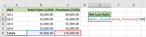
Let’s consider the following dataset showing the total claims a particular insurance company paid out in 2022 and the total premiums the firm earned in the same year.

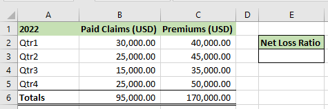
We want to compute the company’s Net Loss Ratio for 2022 and display it in cell E3.

We use the steps below:

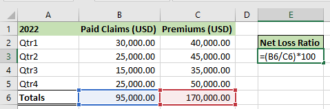
1. Select cell E3 and type in the following formula:

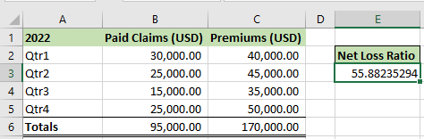
2. Press Enter.

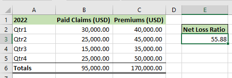
The Net Loss Ratio expressed as a percentage is shown in cell E3.

3. Select cell E3 and click Home >> Number >> Decrease Decimal several times to decrease the decimal numbers of the Net Loss Ratio to two.

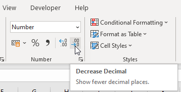
The Net Loss Ratio with two decimal places is displayed in cell E3.

The ratio indicates that the insurance company spent 55.88% of each premium dollar in 2022 to settle claims and retained 44.12% as profit.

Use Named Ranges in Excel’s Net Loss Ratio Formula

Instead of using cell references, we can use named ranges in Excel’s Net Loss Ratio formula. Named ranges will make the formula more readable.

We can name cell B6 containing the total paid claims, “Net Losses,” and cell C6, total earned premiums, “Earned Premiums.”

Name Cells B6 and C6

We use the following steps to name cells B6 and C6:

1. Select cell B6.
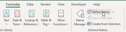
2. Click Formulas >> Define Names >> Define Name.

3. On the New Name dialog box, type Net_Losses on the Name box and click OK.

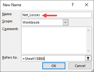
Notice that there should be no spaces in the range name.

4. Select cell C6 and click Formulas >> Define Names >> Define Name.
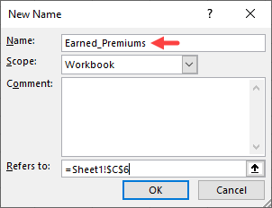
5. On the New Name dialog box, type Earned_Premiums on the Name box and click OK.

Use the Named Ranges in the Net Loss Ratio Formula

Now we can use the named ranges in the formula using the below steps:

1. Select cell E3 and type in the below formula:

Notice that the full name appears in the drop-down as you begin to type the name Net_Losses.

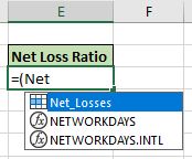
Instead of continuing to type the name, press the tab key to enter the name.

2. Press Enter.

The Net Loss Ratio expressed as a percentage is displayed in cell E3.

Conclusion

This tutorial showed how to use the Net Loss Ratio formula in Excel. In addition, it explained how to use named ranges instead of cell references to make the formula more readable. We hope you found the tutorial helpful.