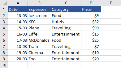
Let’s take a look at the current example. You are traveling the world and there is a list of expenses you made. Each expense is divided into categories. You want to highlight only two categories: Entertainment and Food. One of the few ways you can do it is to use a formula in a conditional formatting rule.
The OR function in the conditional formatting
- Highlight cells from C2 to C9 to choose all dates in the category header.
- Navigate to Home >> Styles >> Conditional Formatting >> New Rule.
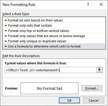
- Click “Use formula to determine which cells to format”.
- Inside “Format values where this formula is true”, type this formula: =OR(c2=”food”,c2=”entertainment”)
When you compare values using the comparison operator, you don’t have to pay attention to capitalization.
- Click the Format button.
- From a new window, click the Fill tab and choose a color. Click OK to confirm.
- Click OK to apply the new rule.
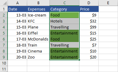
The table is formatted and the “Food” and “Entertainment” categories are highlighted.