You can use the SUM function to add a range of cells in Excel. However, if some cells in the cell range contain errors such as #N/A, #VALUE!, #REF!, #DIV/0!, #NUM!, or #NAME?, the SUM function will return an error instead of a total.
Sometimes you need to know the sum of a cell range even if it contains errors. Therefore, sum up the cell range and ignore any cells that contain errors.
Note: Errors in a worksheet reveal an underlying problem that needs to be addressed; therefore, sum and ignore errors in Excel cautiously.
This tutorial shows three techniques for summing a range and ignoring errors in Excel.
How to Sum and Ignore Errors in Excel
Method #1: Use a Formula Combining the SUM and IFERROR Functions
The SUM function in Excel adds a range of cells or values, but if some cells in the cell range have errors, the function will return an error instead of a total, as seen in the example dataset below, where some cells in column D have the #VALUE! error:
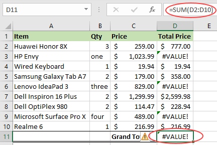
To prevent the SUM function from returning an error value instead of a total, you can use a formula combining the SUM function and the IFERROR functions to ignore the errors and produce a total.
The syntax of the IFERROR function is as follows:
|
1 |
=IFERROR(value,value_if_error) |
The IFERROR function returns value_if_error if the expression is an error. Otherwise, it returns the value of the expression.
About the example dataset, you can use the following steps to sum and ignore errors in column D:
- Select cell D11 and type in the formula below:
|
1 |
=SUM(IFERROR(D2:D10,0)) |
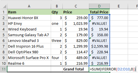
- Press Enter.
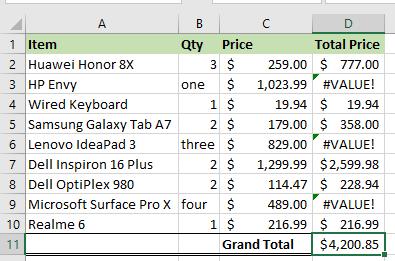
The formula combining the SUM and IFERROR functions returns a total, not an error value.
Explanation of the formula
|
1 |
=SUM(IFERROR(D2:D10,0)) |
The IFERROR function replaces any error value in a cell with a zero value. Otherwise, it returns the value in the cell.
The SUM function finally sums all the values returned by the IFERROR function.
Method #2: Use the SUMIF function
The SUMIF function adds the cells specified by a given condition or criteria.
The syntax of the SUMIF function is as follows:
|
1 |
=SUMIF(range,criteria,[sum_range]) |
We can use the SUMIF function to sum and ignore errors in Excel by specifying in the criteria argument that the values to be added must be equal to or above zero.
We have the following dataset showing a list of electronic items, their quantities, prices, and total prices.

We can use the SUMIF function to determine the total prices of the items and ignore the errors using the below steps:
- Select cell D11 and type in the below formula:
|
1 |
=SUMIF(D2:D10,">=0") |
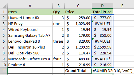
- Press Enter.
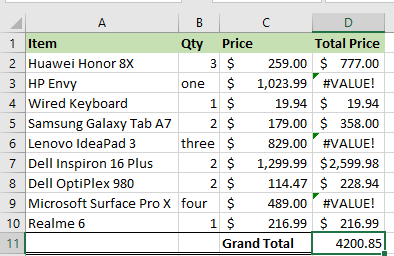
The SUMIF function returns a total, not an error value.
Explanation of the formula
|
1 |
=SUMIF(D2:D10,">=0") |
This formula will add up all the cells in the cell range D2:D10, and any cells that contain errors will be treated as if they have a zero value.
Method #3: Use the AGGREGATE Function
You can sum and ignore errors in Excel by using the AGGREGATE function and configuring it to calculate and ignore errors by setting the function_num argument to 9 and options argument to 6, as shown below:
Set the function_num argument to 9:
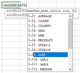
Set the options argument to 6:

Let’s use the AGGREGATE function to sum column D in the following dataset and ignore errors.
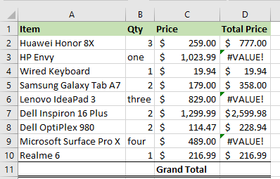
We use the following steps:
- Select cell D11 and type in the below formula:
|
1 |
=AGGREGATE(9,6,D2:D10) |
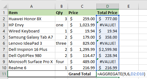
- Press Enter.
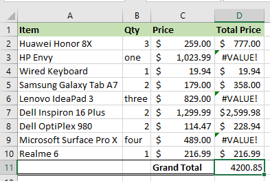
The AGGREGATE formula sums the cell range D2:D10 and ignores all the errors in the cell range.
Conclusion
Sometimes you need to know the sum of a cell range even if it contains errors. Therefore, sum up the cell range and ignore any cells that contain errors.
This tutorial showed three methods for summing and ignoring errors in Excel. This tutorial showed three methods for summing and ignoring errors in Excel. The techniques are:
- The use of a formula combining the SUM and IFERROR functions.
- The use of the SUMIF function.
- The use of the AGGREGATE function.
We hope you found the tutorial helpful.
