Use SUMIF with Wildcard Characters in Excel

The SUMIF formula in Excel is simple to use. It is very intuitive for every user. It has three parameters: range, criteria, and sum_range.

In the example below, we will show how to combine this formula and wildcard characters.

Use SUMIF with the Wildcard Characters

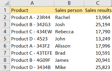
For our example, we will use a list of products, salespersons, and sales results for a certain product:

In terms of wildcards, there are two types of them that can be used: an asterisk (*) and a question mark (?). We can use asterisks before, after, or we can surround the criteria to replace any existing characters. We can use question marks as a representation of a position in criteria where we want to allow the character.

We will use these in the following examples:

1. Let’s assume that we want to find out the sales results for Product A, regardless of the product code.

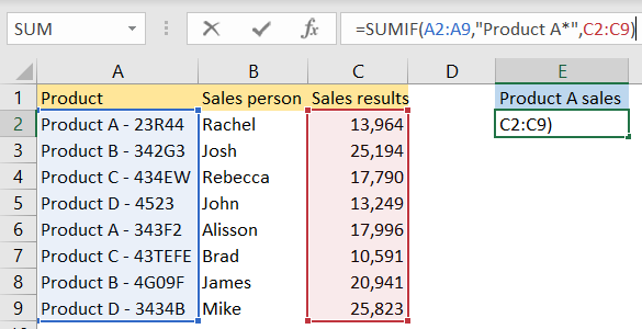
To do this, we will insert the following formula in cell E2:

This is what the formula looks like in the sheet:

And the result we get will be $31,960, which means that both numbers from cell C2 and cell C6 will be included. In this formula, we only used an asterisk at the end of the name of the product we need. It replaces everything that comes after “Product A”, regardless of what it is. Asterisk, unlike the question mark, replaces multiple characters.

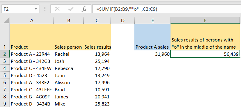
2. Suppose that we want to find out the sales results of all the persons that have the letter “o” somewhere in the middle of their name. From the look of it, we can see that Josh, John, and Alisson should be included in the calculation.

We will put the following formula in cell F2:

And will get the following result:

As already said, an asterisk replaces multiple characters, and in our case, we use two asterisks to replace the text before and after the letter “o”.

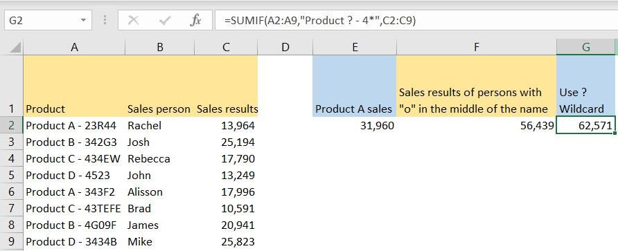
3. Now suppose that we want to know the sales results for every product that has a code that starts with the number 4.

We can use a “?” wildcard for this purpose. We will insert the following code in cell G2:

What this code does, is it takes all the Products: whether it is a product A, B, C, or any other, for that matter, in the calculation. It could be a number as well. We then use an asterisk to find all the products with code number 4. This is our end result:

To conclude, we can use wildcards to replace multiple characters before and after a certain text, and a question mark to replace one character. They can be very convenient in combination with SUMIF, COUNTIF, and many other formulas.