VLOOKUP with CONCATENATE in Excel

One of the most useful functions in Excel is VLOOKUP. It can be combined with different functions as well.

In the example below, we will show how to combine VLOOKUP with CONCATENATE function.

Combine VLOOKUP and CONCATENATE

First thing first, we will break down these two formulas:

1. VLOOKUP formula is an Excel function with which you can find a certain value by looking for it vertically from the range.

It has three required parameters and one optional:

• lookup_value (a value that we are searching for. In our example, this is where the CONCATENATE formula will go).
• table_array (the table, or the range in which we want to find our value. The same value as in lookup_value must be located in the first column of the table array).
• col_index_number (this is the number of the column in the table from which we want to derive the data from. If our lookup value is located in the fourth row of our table, and we choose column number three, this means that we will get the value from this cell returned).
• range_lookup (this is an optional parameter that helps us define if we want the find the exact match of our lookup value, or if we want to find an approximate match. The exact match is FALSE, and the approximate value is TRUE. If we do not choose any option, the default value will be set to TRUE).

2. The CONCATENATE function is a text function that joins two or more strings into one string.

It can have multiple parameters, i.e. strings that we want to join together.

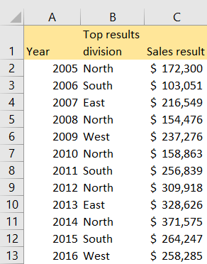
For our example, we will use the list of yearly results for different divisions in terms of sales achieved:

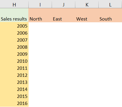
From this table, let us suppose that we want to create a table where the years would be shown in rows, while the division would be shown in columns, like a matrix:

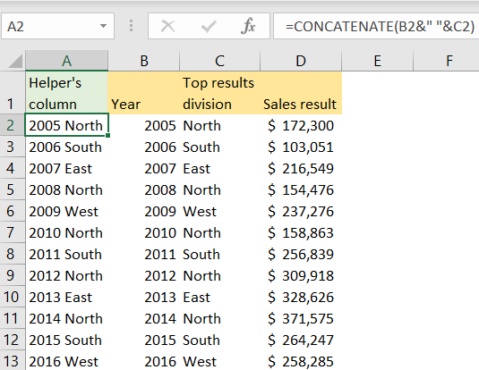
To achieve this with the VLOOKUP function, we need to create the helper column and use CONCATENATE to merge years and divisions in one cell. We will add a column that will take place of our column A, and will insert the formula:

We will drag the formula till the end of the table, and this will be the result:

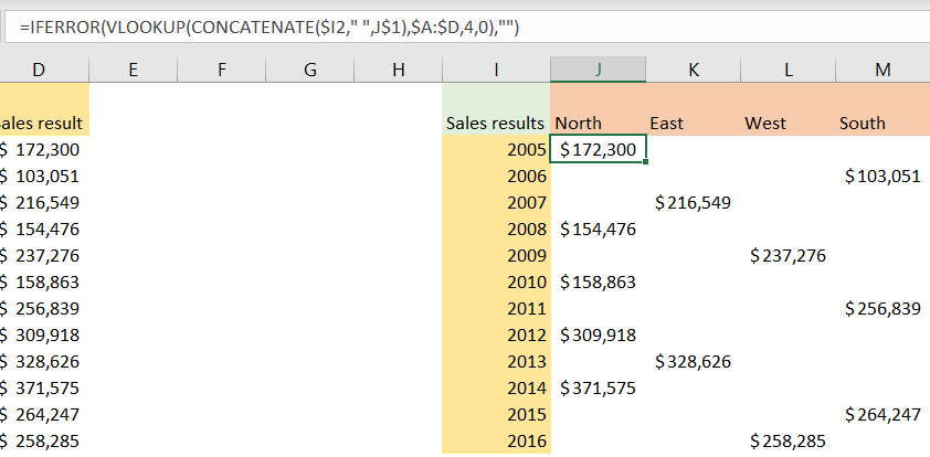
To fill our matrix, we need to combine VLOOKUP and CONCATENATE formulas in one. As said, we will use the CONCATENATE as a range lookup part of this large formula. This is the formula we will insert in cell J2:

First, we use the IFFERROR formula so that we do not return “#N/A” results. CONCATENATE will combine year and division. Years will be locked by column, so only the rows will change, while the divisions will be locked by rows, so only columns will change.

We will use our existing table as a table array (we will lock it as well) and will look for sales results. Dragging the formula throughout our new table will give us the following results:

In conclusion, the best way to combine the VLOOKUP formula with CONCATENATE is to use the cells that are the direct product of cells merging as a lookup value.