As with anything related to Excel, with any possible scenario or formula, there is an option to do it faster and automate it with VBA.
The same thing applies when we discuss filtering options in Excel. In the example below, we will show how to use filters in VBA in multiple scenarios.
Filter Multiple Columns by Multiple Criteria
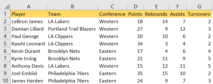
For our example, we will use the list of NBA players, and their statistics from one night of basketball: points, rebounds, assists, and turnovers:

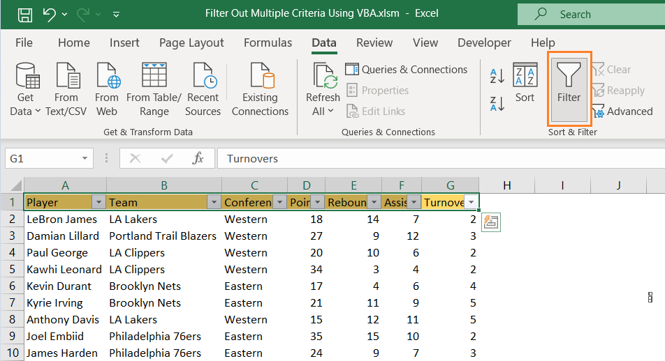
Now, if we would want to filter all the players from the Western Conference that scored 30 or more points, we could do that by going to selecting the data in the first row, and then going to Data >> Sort & Filter >> Filter:

We would go on now to choose what we want to filter out. Of course, we can always use VBA to achieve the same results.
We will open the VBA by clicking ALT + F11 on our keyboard, and then go to the Insert tab on the window that appears, and choose Module:

In the window that appears on the right side, we will insert the following code:
|
1 2 3 4 5 6 |
Sub ColumnsMultipleCriteria() With Range("A1:G10") .AutoFilter Field:=3, Criteria1:="Western" .AutoFilter Field:=4, Criteria1:=">=30" End With End Sub |
This code uses the With function to define the action in the desired range. Our range is A1:G10, and we use an auto filter to declare the fields and criteria that we want to use. Our fields will be numbers 3 and 4, and the requirements for Field 3 (which is basically our column C) will be Western, and for Field 4 (column D) will be over 30.
We execute the code by pressing F5 on our keyboard, while in the module, and we get the following result:

Filter Column by Multiple Criteria with Operator And
In our previous example, we wanted to filter two criteria in two columns. For the next one, we will presume that we want to filter multiple criteria but in the same column.
For this, we will filter all the players (regardless of the conference) that have scored more than 20, and less than 30 points.
Our code for this scenario will be:
|
1 2 3 4 |
Sub OneColumnMultipleCriteria() Range("A1:G10").AutoFilter Field:=4, _ Criteria1:=">20", Operator:=xlAnd, Criteria2:="<=30" End Sub |
This code looks at our table, finds the column with points, and then defines the criteria, which is more or equal to 20 points, and less or equal to 30 points.
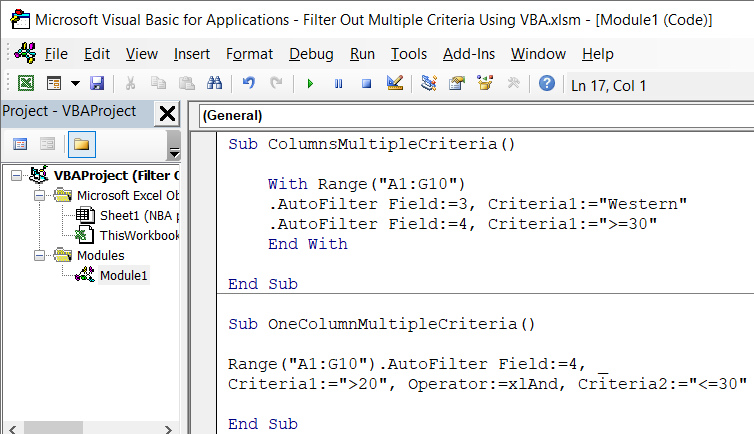
This is what the two codes look like in the module:

You need to have in mind that we already have one filter (the one from the first case) active, so if we would go on and press F5 while in the second code, we would end up with this result:

Since our original tables show that we have three players in this category, our code needs a little tweak. We will add the following part to it:
|
1 2 3 |
If ActiveSheet.AutoFilterMode Then ActiveSheet.AutoFilterMode = FALSE End If |
To make it work. This part only checks if we already have a filter on our active sheet. If yes, then we will remove it.
When we execute the whole code again:
|
1 2 3 4 5 6 7 |
Sub OneColumnMultipleCriteria() If ActiveSheet.AutoFilterMode Then ActiveSheet.AutoFilterMode = FALSE End If Range("A1:G10").AutoFilter Field:=4, _ Criteria1:=">20", Operator:=xlAnd, Criteria2:="<=30" End Sub |
We will get the proper result:

Filter Column by Multiple Criteria with Operator Or
We can also use the “OR” operator to filter out the results if needed. For example, let’s say that we want to filter out all the players that had less than five or more than 13 rebounds.
This will be our formula:
|
1 2 3 4 5 6 7 |
Sub OneColumnMultipleCriteriaOrOperator() If ActiveSheet.AutoFilterMode Then ActiveSheet.AutoFilterMode = FALSE End If Range("A1:G10").AutoFilter Field:=5, _ Criteria1:="<5", Operator:=xlOr, Criteria2:=">13" End Sub |
It is basically the same one as with the “AND” operator, but we are now filtering the results for column E (field number 5). When we execute the code, this is the result we get:

