You have probably heard about Vlookup and Hlookup functions in Excel. Vlookup is short for Vertical Lookup. With it, we can search for a particular value in our column, to return a value from a different column but in the same row. Hlookup is short for Horizontal Lookup and it does a similar thing, with the difference it searches for a value in a row, not in a column.
With the development of Office 365, a new lookup option was introduced- Xlookup. So far, it is only available in Office 365. Its main advantage is that regardless of where the lookup value is found (in a row or a column) it returns the proper value. In the example below, we will show how the Xlookup works, and how it integrates with Visual Basic for Applications (VBA).
How Xlookup Works
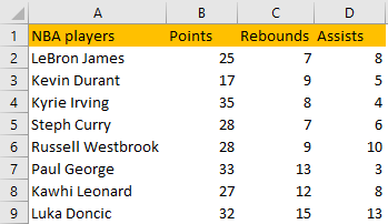
Xlookup can be used to replace both Vlookup and Hlookup. To show the replacement for Vlookup we will first create the table with NBA players and their statistics from several categories (points, rebounds, and assists):
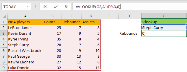
Let us presume now that we want to extract the rebounds for Steph Curry from this table. We will first use Vlookup for this purpose. In cell G1 we will write “Vlookup” and in cell G2 we write Steph Curry. In cell G3 we will write down the following formula:
|
1 |
=VLOOKUP(G2,A1:D9,3,0) |
This is what our formula looks like in the worksheet:
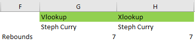
We can use Xlookup for the same purpose. Our formula in cell H3 will do just that. This is what we will write in cell H3:
|
1 |
=XLOOKUP(H2,A1:A9,C1:C9) |
Cell H2 in the formula represents lookup_value (Steph Curry), range A1:A9 stands for lookup_array (where our value is found), and range C1:C9 refers to return_array (the data that we want to show).
When we insert both of these formulas, we will have the same results- which is number 7:
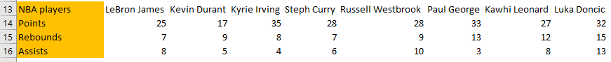
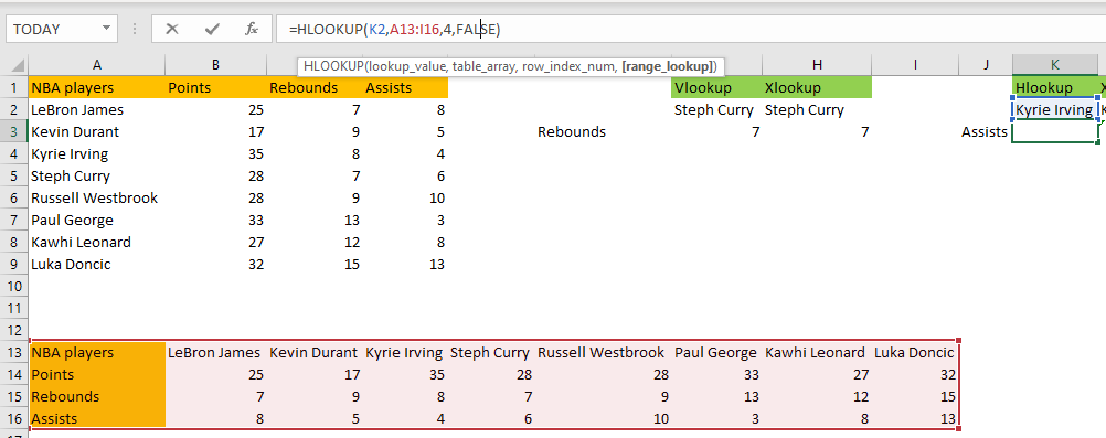
The usefulness of Xlookup lies in the fact that it can be used to replace Hlookup as well. To show this, we will create the horizontal table with the same data, in which points, rebounds, and assists will be in different rows, not different columns:
Now let us say that we want to extract the number of assists for Kyrie Irving. We will do this by using Hlookup. Our formula will be as follows:
|
1 |
=HLOOKUP(K2,A13:I16,4,FALSE) |
Cell K2 represents our lookup_value (Kyrie Irving), range A13:I16 represents the whole table, while number 4 stands for the row where our data is located in the table (assists). We use FALSE for range_lookup to find the exact value.
This is what our formula looks like in the worksheet:
We can use Xlookup for the same purpose, i.e. to extract the same information. Our formula will be as follows:
|
1 |
=XLOOKUP(L2,A13:I13,A16:I16) |
Cell L2 is lookup_value (Kyrie Irving), range A13:I13 refers to lookup_array (all players), and range A16:I16 represents return_array (range where our data is located).
This is what this formula looks like in the worksheet:
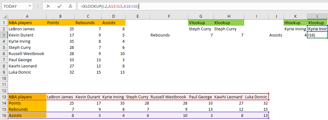
We will get the same value for Kyrie Irving’s assist number- number 4.
All that is shown above can be used in Visual Basic for Application (VBA) for purpose of automation. We will show how to do that below.
Use Xlookup in Vba
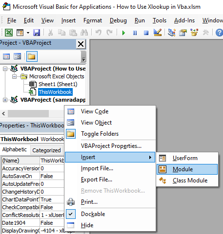
To use VBA, we first need to access it. To do that, we will click on ALT + F11 on our keyboard. On the window that appears, we will right-click on the left window, and go to Insert >> Module:
When we click on this, a new blank window will appear on the right side of the screen. There are two ways to call for Xlookup in VBA. We can use:
- Application.WorksheetFunction.Xlookup
- Application.Xlookup
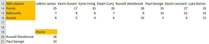
We will find points for Russell Westbrook (we will put his name in cell A20) and for Paul George (cell A21) using VBA and our created tables. These two cells will be used as lookup values in our formula.
We will first search for Russell Westbrook’s points in our first table. This will be our sub-routine:
|
1 2 3 4 |
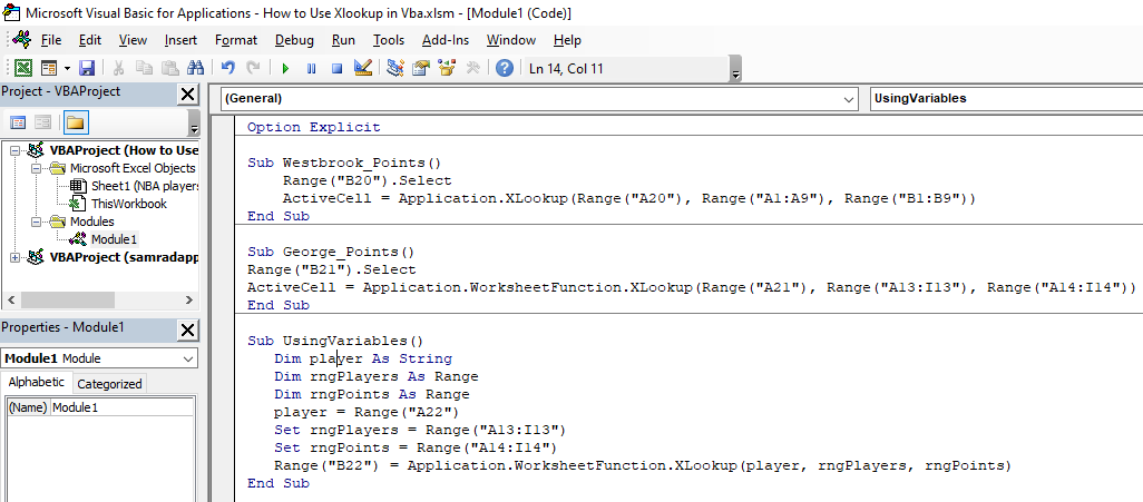
Sub Westbrook_Points() Range("B20").Select ActiveCell = Application.XLookup(Range("A20"), Range("A1:A9"), Range("B1:B9")) End Sub |
First, we position ourselves in cell B20. Then we insert our formula in this cell, using cell A20 as a lookup, range A1:A9 as lookup_array, and range B1:B9 as return_array.
When we run our code by pressing F5 while in the module, we will get the correct result in cell B20:
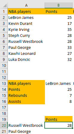
When comparing values in cell B6 and cell B20, we will see that they are the same.
For the code above, we used Application.Xlookup. As said, Application.WorksheetFunction.XLookup can also be used to achieve the same results.
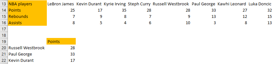
We will write down the following code to extract Paul George’s points from the second table we have (table with horizontal data):
|
1 2 3 4 |
Sub George_Points() Range("B21").Select ActiveCell = Application.WorksheetFunction.XLookup(Range("A21"), Range("A13:I13"), Range("A14:I14")) End Sub |
This formula is pretty similar to the one above, with the difference it imitates Hlookup. We first position ourselves on cell B21, and then we define lookup_value (cell A21- Paul George), lookup_array (range A13:I13– where all the player names are found), and return_array (range A14:I14– where data for points are located).
When we execute the code by pressing F5 on our keyboard (while in the module, and while located in the code with the pointer), this is the result we will get:
We will get the number 33 for Paul George’s points, which is the same number that can be found in row number 14 beneath the name of Paul George, which is a confirmation that the code is good.
The important note is that we must have the lookup_values written in the worksheet before we run the code.
We can also use variables for our code, to show our code more analytically. We will find the points for Kevin Durant in the second table (lookup_value will be in cell A22), and this will be our code:
|
1 2 3 4 5 6 7 8 9 |
Sub UsingVariables() Dim player As String Dim rngPlayers As Range Dim rngPoints As Range player = Range("A22") Set rngPlayers = Range("A13:I13") Set rngPoints = Range("A14:I14") Range("B22") = Application.WorksheetFunction.XLookup(player, rngPlayers, rngPoints) End Sub |
The code above first declares three variables: player, rngPlayers, and rngPoints. Then we set these variables. The player is cell A22– which is Kevin Durant, rngPlayers is for players in our table, and rngPoints refers to points.
When we execute the code, this is what we will end up with:
This is what our code looks like in the module:
We can also create the code with the Application.InputBox and ask users to input all the values that they want, i.e. to choose all the parameters, but we will not show this in this example.