We can often find ourselves in a situation where we need to manipulate percentages in Excel. It is so much easier, as for dates, to just observe the percentages as for what they are- numbers.
In the text below, we will show how to change cell color based on percentages.
Change Cell Color with Formula
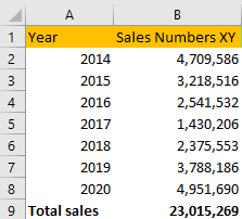
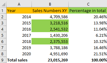
For the example, we will use the table with sales numbers for company XY for the period from 2014 to 2020:
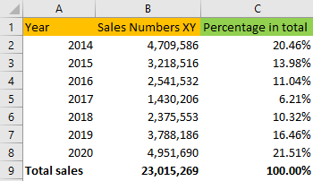
To see the percentage of each year in total sales, all we need to do is divide the number of sales for each year by total sales:
Our formula in cell C2 will be:
|
1 |
=B2/$B$9 |
And we will drag this formula until the ninth row. Our table now looks like this.
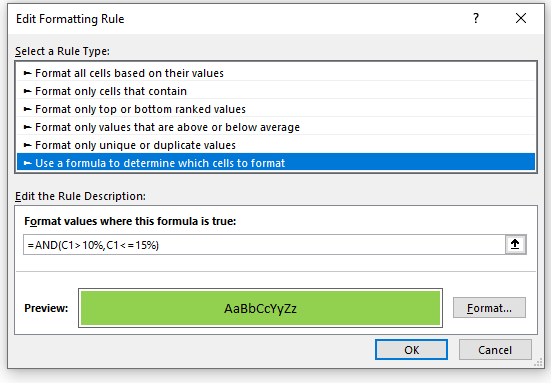
Now let us say that we want to highlight the numbers in column B that takes between 10 and 15 percent of total sales.
We need to use a formula for this. We will select column B, go to the Home tab >> Styles >> Conditional Formatting >> New Rule:
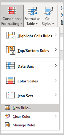
When we click on it, on the pop-up window that appears, we will choose the last option- Use a formula to define which cells to format.
Then we will input our formula:
|
1 |
=AND(C1>10%,C1<=15%) |
Finally, we will define that these cells should be highlighted in green:
Now we will have our values in column B highlighted as defined:
Change Cell Color with Other Conditional Formatting Rules
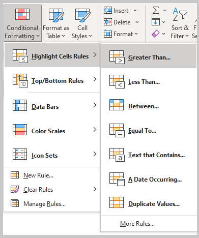
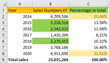
We can manipulate formatting styles and colors with other conditional formatting rules as well. To show this in a particular example, we will highlight all the cells in column C that are larger than 20 percent.
To do this, we need to select range C2:C8 (to exclude the total sales) and then go to Conditional Formatting >> Highlight Cells Rules >> Greater Than:
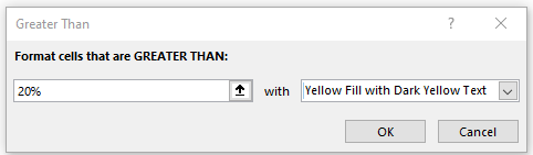
On a pop-up window that appears, we will input desired number (20 percent) and format these cells with yellow color:
Now, our table looks like this:
We could have also left this table intact, and created another IF formula in column D:
|
1 |
=IF(C2<20%,"Bad year","Good year") |
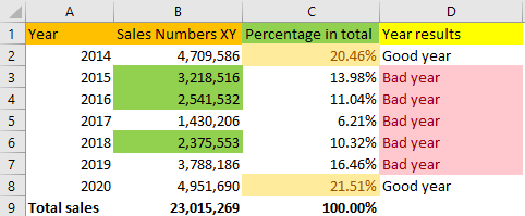
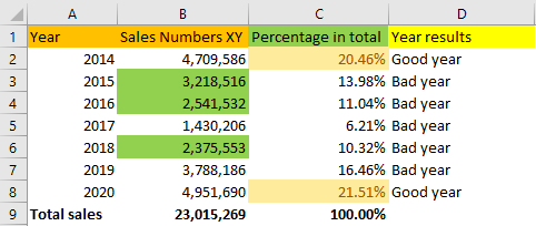
As seen, every year in which less than 20 percent of total sales were achieved will be considered to be a bad year, while every other year will be a good year.
The results are as follows:
Now we can use this column to highlight the cells we want. We will highlight all the bad years by going to Conditional Formatting >> Highlight Cells Rules >> Text that Contains:
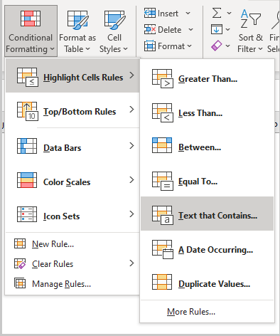
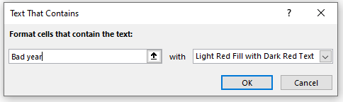
On a pop-up window that appears, we will input desired words: “Bad year”, and highlight them with red color:
Finally, our table looks like this: