We already showed techniques for ordering the items in the Slicer and locking it so it cannot be moved in the Excel file.
In the text below, we are going to present exactly how to hide the Slicer, if ever needed.
Hide a Slicer with Selection Pane
For the example, we will use the standard table that we used before, which consists of NBA players, their teams, conferences, and statistics from several matches.
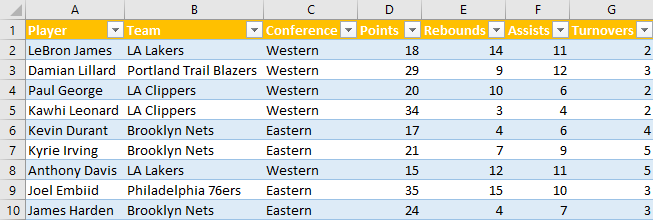
Our data set has 28 rows, but only 10 are presented in the table above.
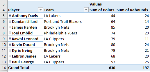
We will create the Pivot Table, put Players and Teams in the Rows field, and sum points and rebounds in the Values field.
Our table looks like this:
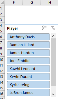
We will create a Slicer with a Player column.
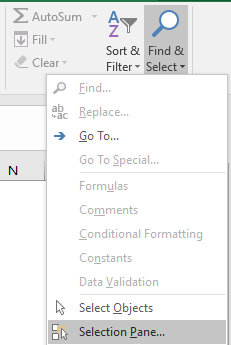
If we want to hide our Slicer, for any reason, our first option is to click on it, then go to Home >> Editing >> Find & Select >> Selection Pane:
When we click on it, we will have a window appears on the right side of our screen:

You will notice that we only have our Player column in the selection pane, along with the little eye symbol to the right.
In order to hide our Slicer, all we have to do is click that eye symbol. Now, the eye will conveniently be closed:

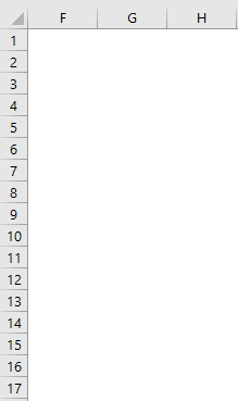
The changes were made for our Slicer too. It was located in the F4:H17 range. Now, these cells are basically empty.
Hide a Slicer with Size and Properties
We will click on the eye symbol again, in order to make our Slicer visible again. There is another way for us to hide the Slicer.
We will right-click on it, then go to Size and Properties:
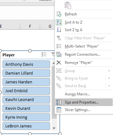
When we click here, the panel will appear on the right of the screen. From it, we will expand Properties and select Move and size with cells option.
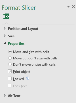
This allows the Slicer to be directly connected with cells in the worksheet. To hide the Slicer, we will now hide the columns in which it is located: E, F, and G.
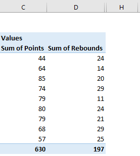
When we hide these columns, our Slicer will be hidden as well.
