Randomness is a lack of pattern or predictability in events. It can be observed in nature, for example in the thermal change or decay of radioactive material. Computers, on the other hand, are things that are designed to eliminate randomness from the results because we want them to be predictable.
For that reason, we can’t really create a list of true random numbers using Excel or any other computer application. What we really mean by saying random, when talking about computers, is a pseudo-random number, a number that is generated using a specific pattern.
To generate a list of pseudo-numbers we need a so-called “seed”. The seed is a number that is used to initialize a pseudo-random number generation.
The repeatability of a pattern is determined by the length of the seed used in the process.
For example, if you use a two-digit seed, the algorithm can produce at most 100 numbers before repeating the cycle. A three-digit seed will expand this number to 1000, 4 digits to 10000, and so on.
Take a look at these two bitmaps. The first one is generated using the random.org website. The site offers true randomization because it uses data generated by a natural process, such as atmospheric noise.
Random bitmap

The second one uses the PHP rand() function. The seed number is not long enough, so we can observe the repeating pattern.
Pseudo-random bitmap

First, take a look at advanced pseudo-random generation and then I will show you how you can use a bit of the VBA code to generate real random numbers.
RAND() function
The most popular way to generate a pseudo-random number is by using the RAND() function. This function doesn’t use any parameter and returns a decimal value between 0 and 1.
|
1 |
=RAND() * (65-18) |
It means: Generate a random number between 0 and 1. Then multiply it by 65 minus 18 (which symbolize the maximum and minimum numbers). Now, the generated value is a number between 0 and 47. Let’s add a minimum number of years, which is 18.
|
1 |
=RAND() * (65-18) + 18 |
Each time you press F9 you will get a sequence of pseudorandom numbers:
29.54275
59.36941
42.83664
21.53878
Of course, no one will say that he has 29,54275 years. Let’s use the ROUND() function to make integers from these numbers.
|
1 |
=ROUND(RAND() * (65-18) + 18, 0) |
Press F9 to generate a list of random numbers between 18 and 65.
38
37
52
59
RANDBETWEEN() function
The easier and faster method to achieve the same result is by using the RANDBETWEEN function(). This function will return an integer value that is between two arguments: the lowest and the highest number. For our example, it will be:
|
1 |
=RANDBETWEEN(18, 65) |
Volatile and static numbers.
The RAND and RANDBETWEEN functions are volatile. It means that each time you change anything in your worksheet the value is recalculated. There are two simple ways you can work around this problem.
- The first one is to copy and paste the generated numbers as values.
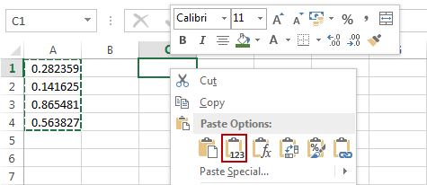
- To use the send method, go to FORMULAS >> Calculation >> Calculation Options and choose Manual. Now, when you change something in the worksheet, the values stay, but when you use the F9 key, the values will be recalculated.
Randomize the list in VBA
If you want your cell not to be recalculated even if you use the F9 key, you have to use VBA.
First, press Left Alt + F11 to open Visual Basic Editor, then create a new module in the project window and enter this code:
|
1 2 3 4 |
Function normalRand() Application.Volatile True normalRand = Rnd End Function |
The code will generate a number. It works the same way as Excel’s RAND function, so the numbers will change every time you change anything in the worksheet.
Change this line:
|
1 |
Application.Volatile True |
To this one:
|
1 |
Application.Volatile False |
Now, when you generate a new number, the value will stay the same. You can also drop this line because of the Application. The volatile procedure is, by default, set to false.
If you want to generate a list of numbers, you can use the AutoFill feature the same way you use it for normal Excel functions.
Random Selection
Example 1: Randomly assign employees
In this example, we will randomly assign workers to work on a project for the next 10 days. This is what the example looks like.
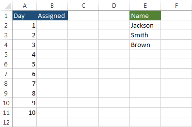
Now, we will try to fill the cells from B2 to B11 with random names from the Name column. In order to do this, we will use the following formula.
|
1 |
=INDEX($E$2:$E$4, RANDBETWEEN(1,3)) |
It will randomly select one name from cells E2 to E4 (absolute cell reference) and insert it into cell B2. Use the AutoFill feature to fill the remaining cells.
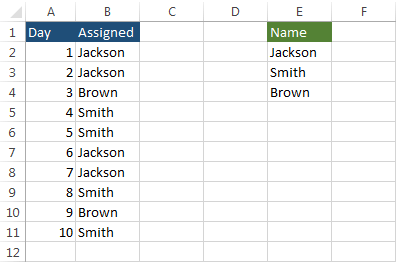
Press F9 to generate a different combination.
Random Sort
I will show you an example you can use to sort a list of values in Excel in a random way.
Example 2:
Suppose you have a list of names of friends you want to call, but you cannot decide which one to call first. In this difficult situation, you decided to sort the names in a random order.
First, fill out the names.
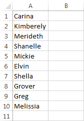
Now change FORMULAS >> Calculation >> Calculation Options to manual and enter =RAND() in cell B1. Fill the rest of the cells (B2:B10), then sort the table by column B. Because we changed the Calculation Options to the manual, the values generated by the RAND function won’t recalculate.
The Random Number Generation tool
To use this tool, first, you need to install the add-in, called the Analysis ToolPak. Go to FILE >> Options >> Add-Ins. Select Analysis Toolpak and click Go…
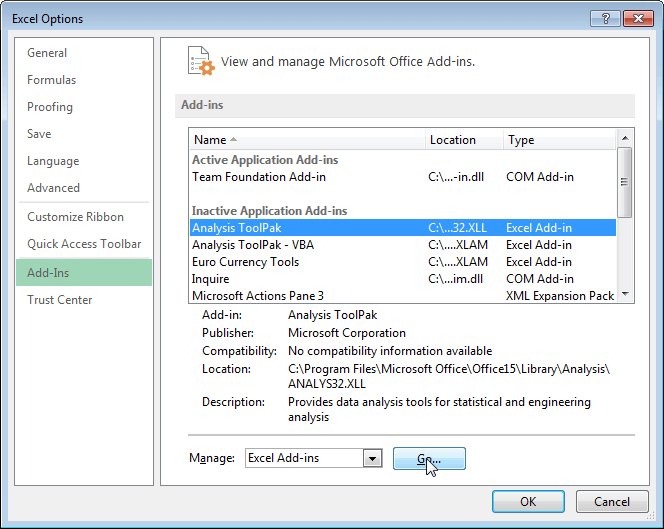
A new window will appear.
Check Analysis Toolpak and click OK.
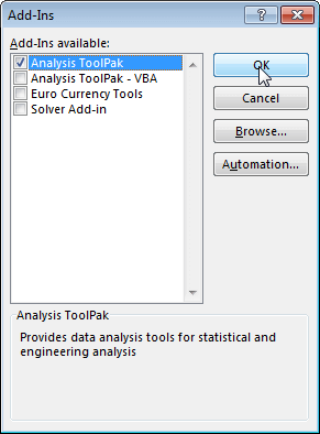
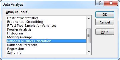
When you do this, a new position will appear in the ribbon, in the data tab. Click the Data Analysis button in DATA >> Analysis. In the new window click “Random Number Generation”.
The new window called the Random Number Generation will appear:
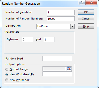
In the Number of Variables you can enter the number of columns and in the Number of Random Numbers the number of rows.
The following types of distributions are available in Analysis Toolpak:
Uniform distribution
The uniform distribution will create random numbers between entered values. In our case, these will be numbers between 10 and 40. This method is similar to the RANDBETWEEN function.
Normal distribution
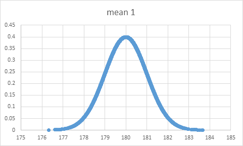
Normal distribution means that most of the numbers are close to average while relatively few examples to the one extreme or the other. When you have enough numbers this distribution will generate a “bell curve” chart.
Here, we have two textboxes: mean and standard deviation.
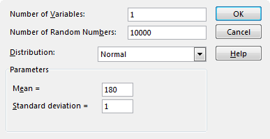
Let’s create two examples, one with a mean that equals 1 and the second one with a mean that equals 3. The mean will represent the average height of men. Let’s suppose that the standard height for men is 180 cm (about 6 feet).
Example 3:
We will create 10000 numbers in one row. Fill text boxes as shown in the image below.
Sort the results. In cell B1 enter the following formula.
|
1 |
=NORM.DIST(A1,180,1,FALSE) |
Click the bottom right corner of the cell to fill in other cells.
Select all the cells and choose INSERT >> Charts >> Recommended Charts. Excel chose a scatter chart. It will be great for the data. Because we have 10 thousand numbers it will look like a line chart in such a small space. But as you can see we have one extreme to the left, so we can see this is a scatter chart.
Example 4:
Change the mean to 3, generate 10 thousand results and see how the chart differs from the previous one.
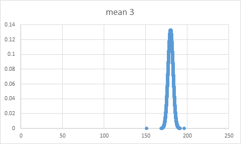
It may seem steeper than the previous one. But take a look at the scale of the x-axis.
The results in both charts are between 150 and 200. Now change the scale. To do this, right-click on the x-axis and select the format axis.

Now, as you can see the higher the mean, the flatter the chart.
Bernoulli distribution
Example 5:
A good example of Bernoulli distribution is tossing a coin. You have a 50% chance of throwing each side of a coin. So in this example, you set the probability to 50% (0.5).
Example 6:
Michael Jordan’s average effectiveness of free throws was 83.5% (.835). Set this parameter in the text box to generate a series of numbers.
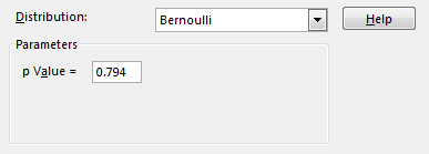
You will get a series of numbers where about 83.5% will be successes (1) and about 16.5% failures (0).
The more numbers you generate the result will be closer to this number.
Binomial distribution
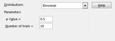
In the Bernoulli distribution, I wrote that the more numbers you generate, the result will be closer to the p Value you chose. In Binomial distribution, you can set two values, the p Value, which is the probability of success, and the number of trials.
Example 7:
We use coin flipping as an example. We use 10 trials and generate 6 results.

Because we used only 10 tries, the results are far from 50%.
Example 8:
Now let’s set the number of trials to 100.

Now the numbers are much closer to 50%- between 46% and 54%.
Example 9:
In the last example let’s use 10000 trials.

Because we used a lot of tries the numbers are much closer to 50%- between 49.71% to 51.34%.
Poisson function
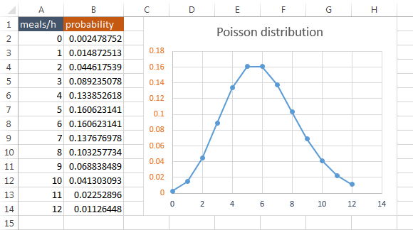
First, let’s talk about the POISSON function. This function will predict the probability of occurring the exact number of events.
Look at the following example:
Example 10:
Let’s say that a restaurant on average sells 6 meals an hour. You want to know what is the probability of selling a particular number of meals.
Fill cells from A2 to A14 with numbers. In cell B2 enter the following formula
|
1 |
=POISSON.DIST(A2,6,FALSE) |
This means: checking the probability of serving a meal in cell A2 when the average number of meals is 6.
Insert the recommended chart to visualize the chances.
Poisson distribution
Now we use the Poisson distribution in the Random Number Generator.
Example 11:
Fill text boxes, as shown in the image below.
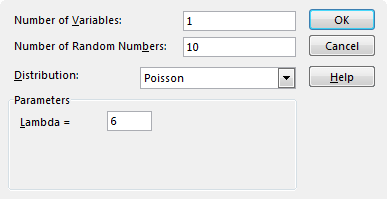
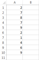
The application will generate 10 numbers where the average number of meals is six. It will take into account the probability of the POISSON function.
I received the following results.
Patterned Distribution
This distribution is called semi-random distribution because it’s more like a tool to fill a series of numbers than a random numbers generator. A number of variables and a Number of Random Numbers are not important in this distribution.
Let’s fill in the numbers as shown in the image below.
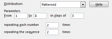
This will give us the following result.
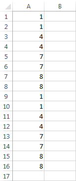
Let’s analyze this example.
The program creates numbers from 1 to 8 in steps of 3. This means that it will create numbers: 1, 4, 7, and 8. It created 8 instead of 10 because this is the last number. Excel will repeat each number twice, so we will get 1, 1, 4, 4, 7, 7, 8, 8. The last thing to do is to repeat the sequence twice. We will get the following results: 1, 1, 4, 4, 7, 7, 8, 8, 1, 1, 4, 4, 7, 7, 8, 8. And that’s our result.
Discrete distribution
The discrete distribution will get values from the two columns you entered in Excel. In the first column are possible outcomes and in the second column are the probabilities of these outcomes.
Example 12:
In the first example, we will create a table with the probability of tossing different numbers of heads. We will use two flips.
Let’s take a look at the possible outcomes:
HH
HT
TH
TT
You have a 25% chance for each flip.
| Number of heads | Probability |
| 0 (TT) | 0.25 |
| 1 (HT, TH) | 0.5 |
| 2 (HH) | 0.25 |
CAUTION
The sum of probability should always be 1.
Create a table and insert the values:
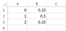
Open the Random Number Generator window and choose a discrete distribution. Select cells from A1 to B3. Generate 10 numbers.
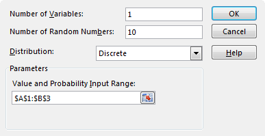
The result in my case is as follows: 1, 1, 1, 1, 1, 0, 0, 1, 2, 1.
Generate real random numbers
We can’t generate real random numbers in Excel, so first, let’s generate these numbers in random.org and then enter them into Excel cells. But we don’t have to do this by hand. Let’s use VBA, so we will be able to generate these numbers with a single click.
Take a look at the following function. More information about functions and subroutines can be found at this link.
|
1 2 3 4 5 6 7 8 9 10 11 12 13 14 15 16 17 |
Function GenRealRand(NUM As Long, MIN As Long, MAX As Long) As Variant Dim obj As Object Dim siteURL As String Dim strResult siteURL = "http://www.random.org/integers/" siteURL = siteURL & "?num=" & NUM & "&min=" & MIN & "&max=" & MAX & "&col=1&base=10&format=plain&rnd=plain" Debug.Print siteURL Set obj = CreateObject("MSXML2.ServerXMLHTTP") With obj .Open "GET", siteURL, False .send strResult = .responseText GenRealRand = Split(strResult, Chr(10)) End With End Function |
1. We created the genRealRand function, which takes 3 arguments.
2-4. Three variables are declared.
6. This is the first part of the link.
7. In the second part, enter the number of values to generate (NUM), minimum values (MIN), and maximum values (MAX) The following URL will generate 10 numbers with values between 1 and 100.
http://www.random.org/integers/?num=10&min=1&max=100&col=1&base=10&format=plain&rnd=plain
9. The object MSXML2.ServerXMLHTTP can be used to retrieve data from a website.
12-13. VBA executes the URL
14. The result from the page is saved to strResult.
15. The function returns a list of numbers separated by a new line (chr(10)).
This function will be executed inside the following subroutine.
|
1 2 3 4 5 6 |
Sub RealRand() Dim numberOfValues As Long Cells.Clear numberOfValues = 10 Range("A1:A" & numberOfValues).Value = Application.Transpose(GenRealRand(numberOfValues, 1, 100)) End Sub |
2. numberOfValues is the number of generated values.
3. Cells.Clear clears worksheet before generating new numbers (be careful to use it inside a new worksheet)
4. The number of values to generate.
5. The number of values that are inserted both into the range and into the GenRealRand function. For example, if numberOfValues is 10, then the function will generate 10 values and insert them into the range (A1:A10).
