Options for the charts in Excel do not only refer to editing and changing the data, but they tend to be limitless. One of the options that we have is to rotate a chart if needed.
In the example below, we will show how to do so with a bar chart.
Rotate a Bar Chart in Excel
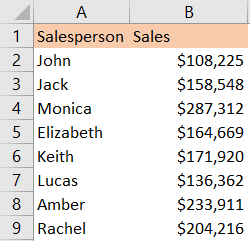
For our example, we will use the sales numbers from several salespersons:
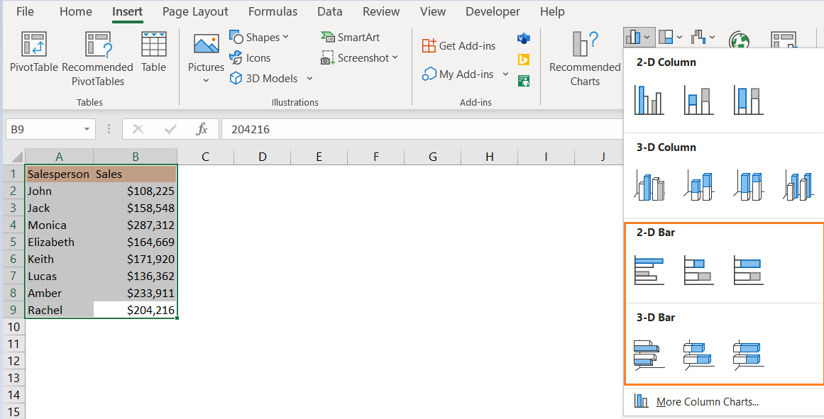
Using this data, we will create a Bar chart, by selecting the data, and then going to Insert >> Charts >> Insert Column or Bar Chart:
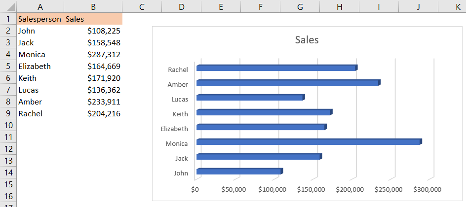
We will choose a 3-D Bar chart, and end up with the following chart:
Using 3-D charts can indicate to people that you really know what you are doing with the charts. If there is a need for rotation of Horizontal and Vertical Axes, we can easily change the order of the values that are found next to these axes.
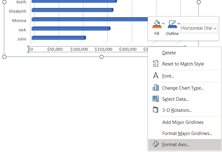
To rotate the chart based on the Horizontal Axis, we will do the following:
Select the horizontal axis, right-click on it, and choose Format Axis:
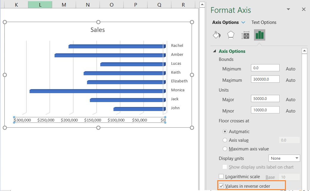
Once we click on it, we will be presented with the new window on the right side. In this window, we will choose Axis Options, and then click on Values in Reverse Order checkbox:
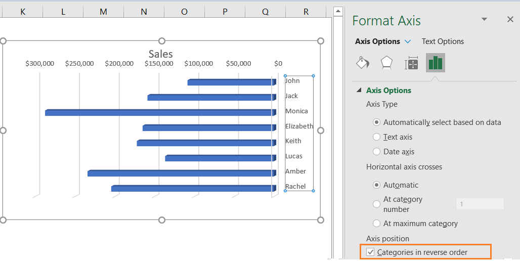
We can do the same thing for Vertical axis as well. We will follow the same steps (right-click on vertical axis, and then go to Axis options) only this time, we will choose Categories in reverse order:
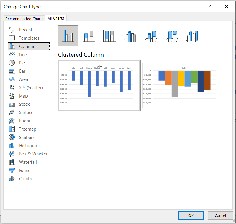
Another simple way to rotate the Bar chart is to actually change it to the Column chart. We do that by right-clicking on the chart, and then choosing Change Chart Type:
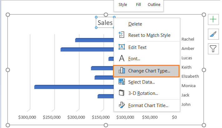
In the dialog box that appears, we will choose Column: