So many users are often found Excel frustrating when dealing with things that could be easily handled with a little effort.
One problem that can often happen is that we have some text and numbers in the same cell. In the example below, we will show how to separate them into two different cells.
Split a Cell at Number with Formula
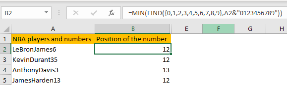
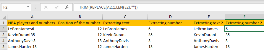
For our example, we will use the list of NBA players and their jersey numbers:

The first thing that we are going to do is to find the position of the number in every particular cell. For this, we are using the following formula:
|
1 |
=MIN(FIND({0,1,2,3,4,5,6,7,8,9},A2&"0123456789")) |
For most of the formulas in which you need to extract or split any kind of information, you need to find the location of your desired separator. When you find this position, it will be easier to use other functions to extract the values.
With the formula above, we will find the position of the number in our range.
FIND function searches for all number positions, and MIN returns us with the first number position.
Now, this part of the function (A2&”0123456789″) concatenates all numbers from 0 to 9 with the original text in cell A2. FIND formula cannot return zero when there is no value, so this is just a way to avoid errors that could occur if the number is not found.
When we drag the formula to the end of our range in column B, we will get the following results:
Now we can use formulas RIGHT or LEFT to extract the text or number, depending on the information we need.
To extract only the text, we will use the following formula:
|
1 |
=LEFT(A2,B2-1) |
And we will get the results as shown below:
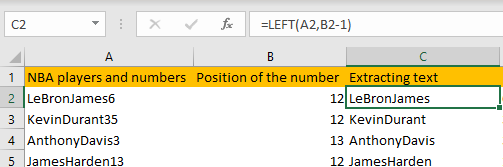
This formula takes characters from the cells in column A, starting from the left. We use the position of the number to define how many characters will be taken from the text. As the number is located at the end of our text, we take the whole number and subtract the number 1 from it (the first number itself).
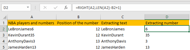
If we would want to show only the numbers now, we would apply the following formula in column C:
|
1 |
=RIGHT(A2,LEN(A2)-B2+1) |
This formula is a mathematical one. If extract what we need from the right side of our text, it sums all the characters in the text in column A, then subtracts the number in column B from this one and adds one character. This way, we will always get desired results:
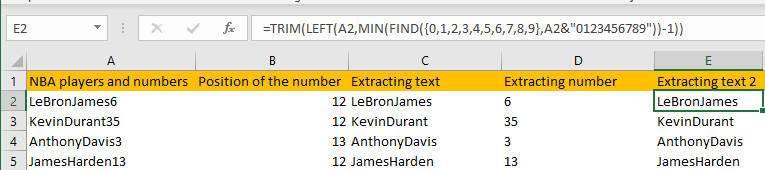
There is also a way to split a cell at the number without knowing the position of the number. To do this, we will apply the following formula in column E:
|
1 |
=TRIM(LEFT(A2,MIN(FIND({0,1,2,3,4,5,6,7,8,9},A2&"0123456789"))-1)) |
The TRIM function removes all spaces from a text string except for single spaces between words. Using this function in a combination with LEFT and the one that we explained above, gives us the following result:
To extract only the numbers, we will use the TRIM function in a combination with REPLACE function. This is what we need to write in column F:
|
1 |
=TRIM(REPLACE(A2,1,LEN(E2),"")) |
We replace the text in column A with several characters in column E, starting from the first character. New text will be the difference between these two columns, which will leave us with numbers only.
This is our result:
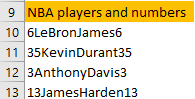
Split a Cell at Number with Text to Columns
For this option, we have to use the help of Microsoft Word as well, so this is not entirely only an Excel tip, but it is pretty easy to use.
We will have the same list of players, but with numbers at the beginning and the end:
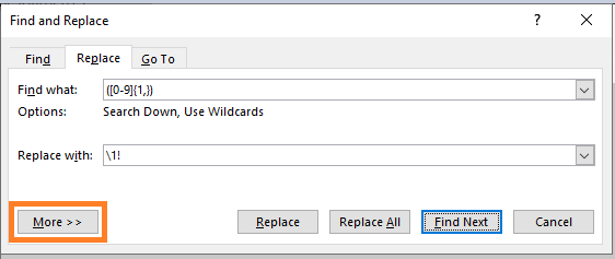
We will open Word and copy and paste this data. After that, we will select the text and click CTRL+H. Then, on the window that appears in Find what part we will type ([0-9]{1,}) and in Replace with we will type \1!.
After that, we will click on More to expand the dialog:
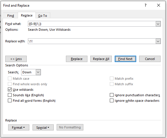
In the dropdown, we will click on the option Use wildcards and click on Replace All:
On the window that appears, we will click OK.

Now we have an exclamation mark right after every number that we have in the text.

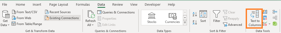
We will copy and paste this into our Excel file. Then we will select this text, go to Data >> Data Tools >> Text to Columns:
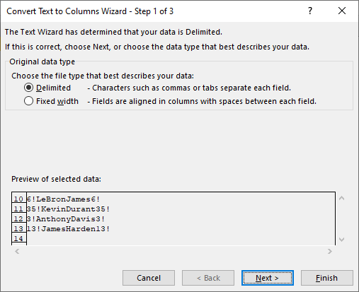
In the dialog that appears, we will choose the Delimited option and click Next:
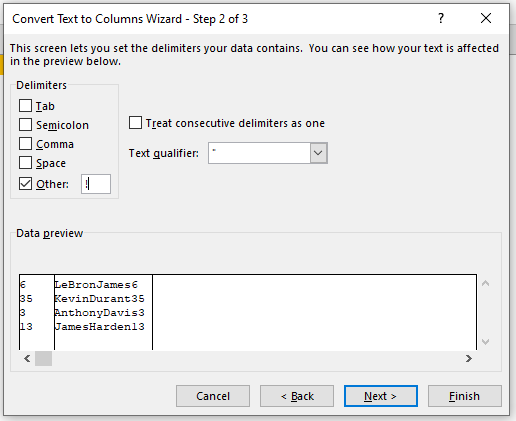
In the next step, we will choose Other in Delimiters, and we will put “!”.
We will click Next and then on the last step, we will click Finish. Now we have the first numbers separated from the rest of the text:

To change the second part, we could select the data in column B, redo our steps, but with the input of !\1 instead of \1!. This will put an exclamation sign in front of our text and solve our problem.