In order to get the value from the cell next to the matching cell, you have to use the vlookup function. This function will look for the value in the specified range and return the value from the chosen column.
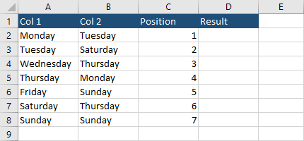
In the following example, there is a list of weekdays from Monday to Sunday and their position.

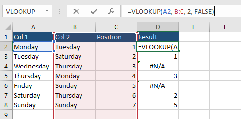
Enter the following code into cell D2 and autofill the rest of the cell in the column.
|
1 |
=VLOOKUP(A2, B:C, 2, FALSE) |

Let’s analyze the code.

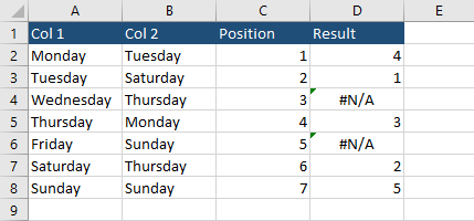
The first occurrence of Monday in Col 2 is in cell B5. Next to Monday is 4. And this value is in cell D2.
Two cells in column D resulted in the #N/A error. If you look closer, you will notice that it happens for Wednesday and Friday. As you can see, they are not present in Col 2.
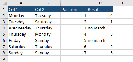
If you want to beautify the code and get rid of these errors, modify the code.
|
1 |
=IFERROR(VLOOKUP(A2, B:C, 2, FALSE), "no match") |

